This article is a part of the Production Machine Learning series of articles.
Features Optimization
Cost and speed are two crucial factors when talking about Production ML—speed results in time to market and speed of reaction to fortunate or an unfortunate event. And the cost is a limit of resources we have.
Production ML pipelines are usually processing vast volumes of data. And data becomes a significant factor influencing speed and cost. The more data we have, the more computing power we need to process it. It is a tangible balance between the resources we allocate and the cost we can bear.
If you take a structured dataset with ten reasonably simple features, each feature would approximately represent 8-10% of data. This means eliminating each feature could decrease the cost and increase the processing speed. I would say that usually, each feature removal could save us from 5% to 30% of the time and money we spend on data processing, model training, and serving. Not bad, right?
This article will discuss simple techniques that will allow us to eliminate features but keep model accuracy metrics on the desired level.
There are three groups of methods that could help us reduce the feature universe:
- Filter methods: primarily uses correlation to define redundant features. Two main rules that this group of methods uses are 1) if two features have a high correlation, then one is redundant; and 2) if a feature has a high correlation with a label, then it is important to keep it. Methods include Pearson correlation and chi2, and others.
- Wrapper methods: consist of forward selection, backward elimination, and recursive elimination. These methods require extensive resources, but the forward selection is the most greedy. In forwards selection, we start from one feature, and we train our model with all possible combinations of two features (one of which is the one we started with). Then three and so on. In backward elimination, we begin from all features and calculate model accuracy with all possible combinations of features minus one. If, for example, we had 20 features, we will calculate model accuracy with all possible combinations of 19 features. Then we remove one more feature and so on. Recursive feature elimination works slightly differently. We select a model and desired number of features. Then we take all features and train the model. We use model embedded methods to identify the importance rank of each feature and remove less important ones. This exercise is repeated until we have the desired number of features.
- Embedded methods: use methods embedded into the model (usually tree-based model like Random Forrest Classifier) to define the feature importance. This group of methods often outperforms the other two because they require less computation and are therefore faster and less expensive. They also provide high accuracy in terms of the best set of features.
All methods share the same goal – identify the optimal set of features that best represent relationships and remove features that do not. By eliminating features, we reduce the resources required for storing and processing the data and minimize the model’s complexity.
This article will show you how to use embedded methods based on Random Forest Classifier and LinearSVC models with L1 regularization. It sounds more complicated than it is.
We will use the same dataset we’ve used in the previous article – Data Ingestion and Validation in Production Machine Learning. Structured Dataset.
Tools
In this article, our main instruments will be pandas and scikit-learn, which you should know from the previous post Data Ingestion and Validation in Production Machine Learning. Structured Dataset. We will also use matplotlib for graphs, and it also should not come as a surprise to you.
We will import the required libraries:
import pandas as pd
import os

from sklearn.model_selection import train_test_split
from sklearn.preprocessing import StandardScaler
from sklearn.ensemble import RandomForestClassifier
from sklearn.svm import LinearSVC
from sklearn.feature_selection import SelectFromModel
from sklearn.metrics import accuracy_score, roc_auc_score, precision_score, recall_score, f1_score

import matplotlib
import matplotlib.pyplot as plt
Let’s take a closer look at methods we are importing from scikit-learn:
- train_test_split: we use it to split the dataset into train and test portions.
- StandardScaler: this method will scale numeric features to have zero mean and unit variance.
- RandomForestClassifier andLinearSVC: are models which embedded methods we will be using to define the importance of features.
- import accuracy_score, roc_auc_score, precision_score, recall_score, f1_score: are Accuracy, ROC, Precision, Recall and F1 Score accordingly.
Load and Prepare Data
First of all, we will download and save our dataset. Then we will read it as a pandas dataframe.
train = './adult.data'
test = './adult.test'

if not os.path.exists(train):
  !wget https://archive.ics.uci.edu/ml/machine-learning-databases/adult/adult.data
  !wget https://archive.ics.uci.edu/ml/machine-learning-databases/adult/adult.test

header_list = ['age', 'workclass', 'fnlwgt', 'education', 'education-num', 'marital-status', 'occupation',
               'relationship', 'race', 'sex', 'capital-gain', 'capital-loss', 'hours-per-week', 'native-country', 'label']

df_feature_engineering = pd.read_csv('./adult.data', names=header_list, skipinitialspace=True)
Let’s take a look at our dataset:
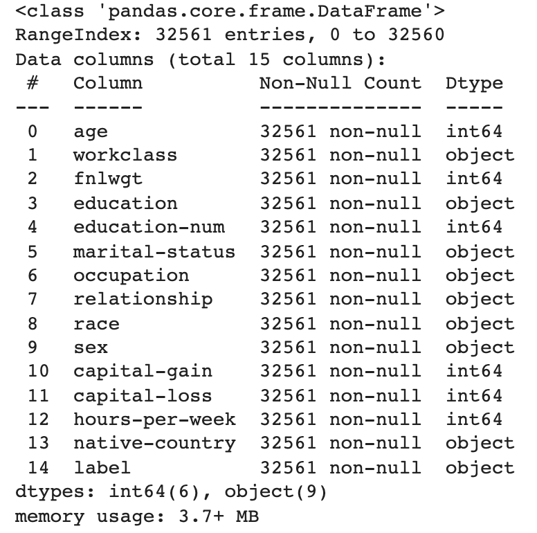
df_feature_engineering.info()When you run the cell with the command, you should see:

Our dataset contains fourteen features, six numeric and eight categorical. To train our model, we will encode our categorical features. Each category will be represented by a number instead of a string.
#list of categorical features
CATEGORICAL_FEATURE_KEYS = [
    'workclass',
    'education',
    'marital-status',
    'occupation',
    'relationship',
    'race',
    'sex',
    'native-country',
    'label'
]
#and label
LABEL_KEY = 'label'
Now we will convert features of type ‘object’ to type ‘category’.
df_feature_engineering[CATEGORICAL_FEATURE_KEYS] = df_feature_engineering[CATEGORICAL_FEATURE_KEYS].astype('category')This is needed for us to be able to use pandas dataframe method, which will encode categorical features:
df_feature_engineering[CATEGORICAL_FEATURE_KEYS] = df_feature_engineering[CATEGORICAL_FEATURE_KEYS].apply(lambda x: x.cat.codes)You can check the updated categories:
df_feature_engineering.head()
The last thing that is left in the preparation phase is to separate features from the label:
X = df_feature_engineering.drop(LABEL_KEY, 1)
Y = df_feature_engineering[LABEL_KEY]
Random Forest Classifier
We will prepare a few functions that we will use. The First would be a function that prepares and fits train data to our Random Forest model.
def feature_importance_model():

  #split dataset into train and test pieces
  X_train, X_test, Y_train, Y_test = train_test_split(X, Y, test_size=0.2, stratify=Y, random_state=123)

  #scale train and test data to zero mean and unit variance
  scaler = StandardScaler().fit(X_train)
  X_train_scaled = scaler.transform(X_train)
  X_test_scaled = scaler.transform(X_test)

  #initialize the model and fir the data
  model = RandomForestClassifier()
  model = model.fit(X_train_scaled, Y_train)

  return model
Following helper function will receive fitted model and feature importance threshold, which will dictate the threshold above which we consider a feature to be important. The function will return names of features that have an importance index above the threshold.
def select_features(model, threshold):

  #use embedded method to indexes of the features importance of which is above threshold
  model = SelectFromModel(model, prefit=True, threshold=threshold)
  feature_idx = model.get_support()

  #get feature names from indexes
  feature_names = df_feature_engineering.drop(LABEL_KEY,1).columns[feature_idx]

  return feature_names
The following small helper function will initiate Random Forest Classifier and fit model with X and Y:
def fit_model(X,Y):

  #initiate model
  model = RandomForestClassifier()

  #fit model on X and Y
  model.fit(X,Y)

  return model
This helper function will calculate model accuracy metrics. It will receive trained model and return model accuracy metrics:
def calculate_accuracy(model, X, Y):

  #get model prediction
  y_pred = model.predict(X)

  #calculate model prediction accuracy metrics
  roc=roc_auc_score(Y, y_pred)
  acc = accuracy_score(Y, y_pred)
  prec = precision_score(Y, y_pred)
  rec = recall_score(Y, y_pred)
  f1 = f1_score(Y, y_pred)

  return acc, roc, prec, rec, f1
Now we will create an orchestration function that will gather the training and evaluation process together:
def train_and_evaluate(X,Y):

  #split train and test set
  X_train, X_test, Y_train, Y_test = train_test_split(X, Y, test_size = 0.2,stratify=Y, random_state = 123)

  #scale and normalize all features.
  scaler = StandardScaler().fit(X_train)
  X_train_scaled = scaler.transform(X_train)
  X_test_scaled = scaler.transform(X_test)

  #train the model
  model = fit_model(X_train_scaled, Y_train)

  #calculate accuracy
  roc, acc, prec, rec, f1 = calculate_accuracy(model, X_test_scaled, Y_test)

  return acc, roc, prec, rec, f1
Following helper function will obtain the model accuracy metrics from the previous helper function and save them to the dataframe so that we can check them later:
def evaluate_model_on_features(X, Y):

  #get metrics
  acc, roc, prec, rec, f1 = train_and_evaluate(X, Y)

  #save metrics to dataframe for display
  display_df = pd.DataFrame([[acc, roc, prec, rec, f1, X.shape[1]]], columns=["Accuracy", "ROC", "Precision", "Recall", "F1 Score", 'Feature Count'])

  return display_df
Now it is time to try our functions:
#calculate evaluation metrics in case of all features
all_features_eval_df = evaluate_model_on_features(X, Y)

#add them to the list of trials
all_features_eval_df.index = ['All features']

#initialize results dataframe
results = all_features_eval_df

#check the results
results.head()
The accuracy of Random Forest Classifier is about 77%:

Now we will perform ten trials with different feature importance thresholds. It will give us a measurement of model accuracy with varying sets of features.
#ten values of importance threshold
IMPORTANCE_THRESHOLD = [0.03, 0.035, 0.04, 0.05, 0.06, 0.065, 0.07, 0.08, 0.085, 0.09]

#loop through each value and run model inference cycle, save accuracy metrics
for threshold_value in IMPORTANCE_THRESHOLD:

  #initiate the model
  model = feature_importance_model()

  #select features that have importance index above the threshold
  important_features = select_features(model, threshold_value)

  #calculate and check model metrics
  feat_imp_eval_df = evaluate_model_on_features(df_feature_engineering[important_features], Y)

  #add list of features to the results of trial
  feat_imp_eval_df.index = [', '.join([ feature for feature in important_features])]

  #append to results and display
  results = results.append(feat_imp_eval_df)
And we can check the results:
results.head(n=11)
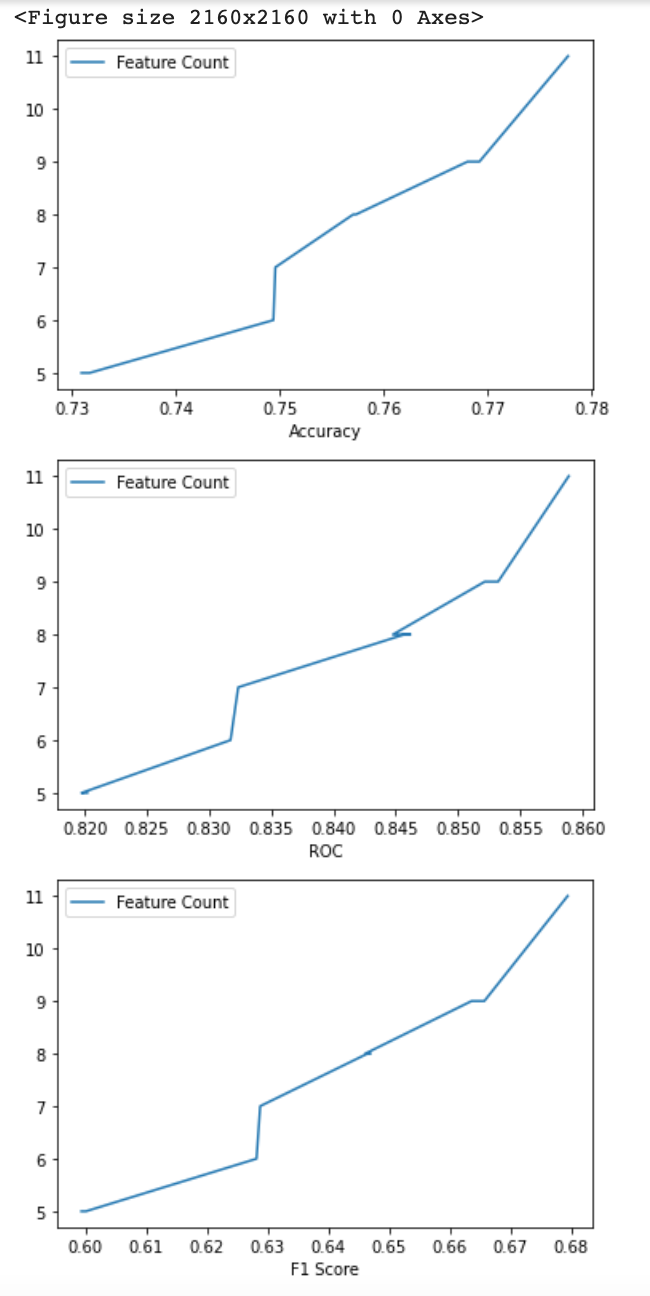
We can remove sex, race, native country features in this case. Accuracy and F1 score both will only drop 0.1%. This could help us save around 20% on storage and processing cost and time. In some cases, we can even go further and tolerate a 1% reduction of accuracy (1.7% reduction in F1 score) but reduce the feature vector to only nine features or even less.
Let’s plot charts showing dependency between the number of features and accuracy:
plt.figure(figsize=(30, 30))
plot_results = results.drop('All features').sort_values('Accuracy', ascending=False)
for label in ['Accuracy', 'ROC', 'F1 Score']:
  plot_results.plot(x=label, y='Feature Count')
  plt.show()
LinearSVC with L1 regularization
In the example above, we set the importance threshold manually. We did it because we were willing to pay for reducing the feature vector with the decrease in model accuracy.
We could also ask a model if it thinks there are non-important features we should get rid of. To do this, we introduce L1 regularization, which will penalize fewer essential features, and therefore guide us towards the list of most important features.
The main helper function requires some changes:
def run_l1_regularization():

  #split train and test set
  X_train, X_test, Y_train, Y_test = train_test_split(X, Y, test_size = 0.2,stratify=Y, random_state = 123)

  #scale and normalize all features.
  scaler = StandardScaler().fit(X_train)
  X_train_scaled = scaler.transform(X_train)
  X_test_scaled = scaler.transform(X_test)

  #get list of features model consider important
  selection = SelectFromModel(LinearSVC(C=1, penalty='l1', dual=False))
  selection.fit(X_train_scaled, Y_train)

  #get feature names
  feature_names = df_feature_engineering.drop(LABEL_KEY,1 ).columns[(selection.get_support())]

  return feature_names

l1reg_feature_names = run_l1_regularization()
Evaluate model accuracy metrics on features selected above:
# Calculate and check model metrics
l1reg_eval_df = evaluate_model_on_features(df_feature_engineering[l1reg_feature_names], Y)
l1reg_eval_df.index = ['L1 Reg']

# Append to results and display
results = results.append(l1reg_eval_df)
results.head(n=12)
We can see that L1 regularization is advising us not to remove features:

Conclusion
Today you saw an example of embedded techniques of feature optimization. Feature optimization is a vital part of Production ML, and I strongly encourage you to try the code above.
I also suggest you check out other methods described in this article because they might produce better results in certain circumstances. Or provide you with more flexibility and control over the decision-making.
Thank you for following me to the end, and may the Force be with You.
Next article in the series – Production ML Data Transformation Pipeline with Apache Beam. Structured Dataset.


