This is the second part of the article. Please find the first part here – Private: Production ML: Deploying model to Virtual Machine. Part 1.
The model
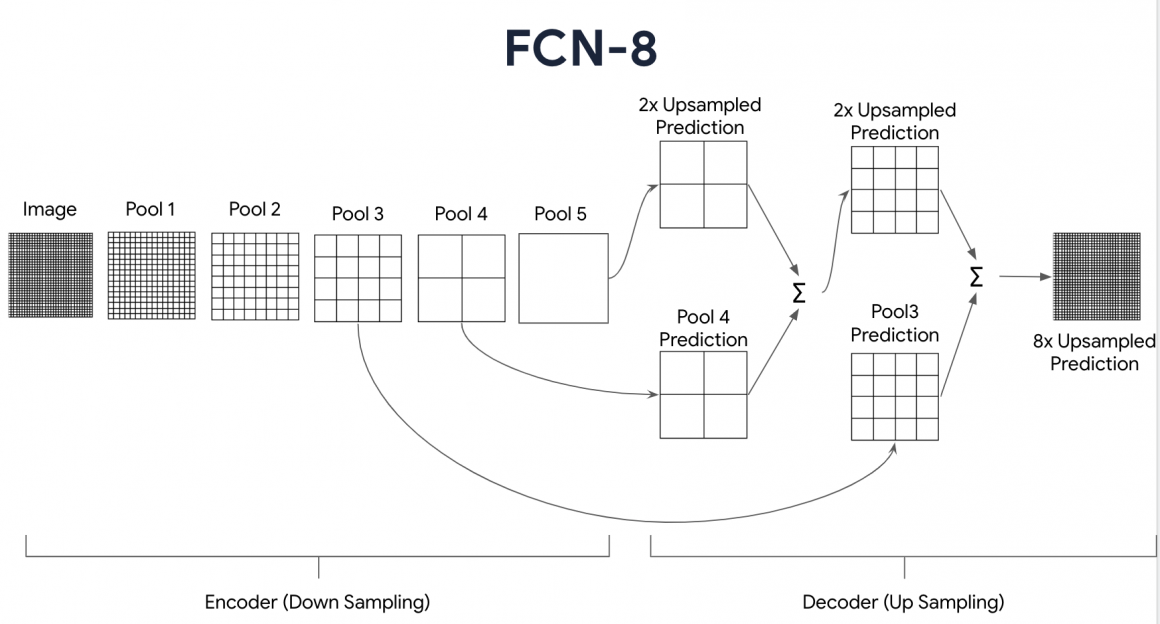
Our model with the fancy name FCN-8 consists of an Encoder and Decoder:

Now we will use the conv_block helper function to generate the downsampling sequence (Encoder) for our model:
def FCN8(input_height=64, input_width=84):
    '''
    Defines the Encoder of the image segmentation model.

    Args:
      input_height (int) -- height of the images
      width (int) -- width of the images

    Returns:
    (tuple of tensors, tensor)
      tuple of tensors -- features extracted at blocks 3 to 5
      tensor -- copy of the input
    '''

    img_input = tf.keras.layers.Input(shape=(input_height,input_width, 1))

    # pad the input image to have dimensions to the nearest power of two
    x = tf.keras.layers.ZeroPadding2D(padding=(0,6))(img_input)

    # Block 1
    x = conv_block(x, 32, 2, 2, 2) #conv_block(input, filters, strides, pooling_size, pool_strides)

    # Block 2
    x = conv_block(x, 64, 2, 2, 2)

    # Block 3
    x = conv_block(x, 128, 2, 2, 2)
    # save the feature map at this stage
    f3 = x

    # Block 4
    x = conv_block(x, 256, 2, 2, 2)
    # save the feature map at this stage
    f4 = x

    # Block 5
    x = conv_block(x, 256, 2, 2, 2)
    # save the feature map at this stage
    f5 = x

    return (f3, f4, f5), img_input
Let’s generate the model we can build so far and see if everything seems fine:
#generate downsampling path
test_convs, test_img_input = FCN8()
test_model = tf.keras.Model(inputs=test_img_input, outputs=[test_convs, test_img_input])

#print model summary
print(test_model.summary())

#delete resources
del test_convs, test_img_input, test_model
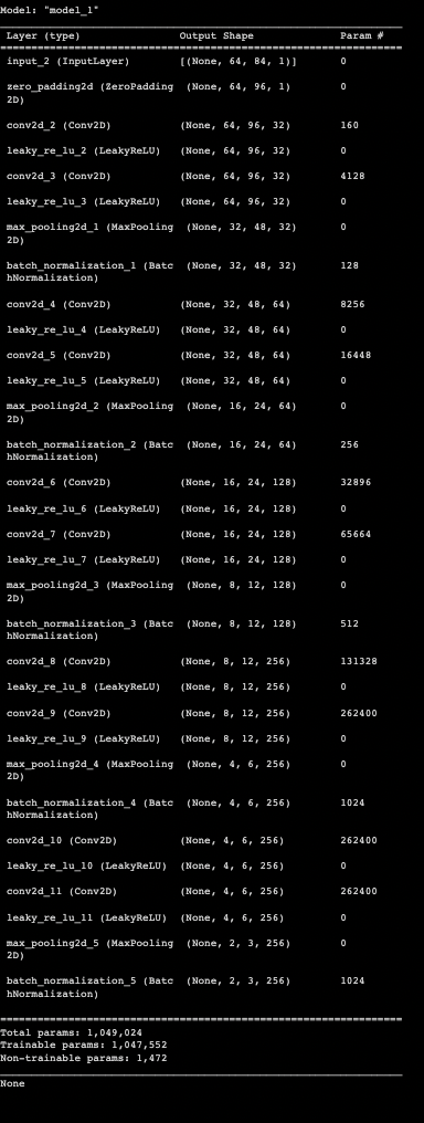
The Encoder summary should look like the following:

And it is time to create the Generator function for the Decoder:
def fcn8_decoder(convs, n_classes):
    '''
    Defines the Decoder of the image segmentation model.

    Args:
      convs (int) -- output from the Encoder
      n_classes (int) -- number or classes in the classification

    Returns:
    Label mask with mask for each pixel in the image
    '''

  # features from the encoder stage
  f3, f4, f5 = convs

  # number of filters
  n = 512

  # add convolutional layers on top of the CNN extractor.
  o = tf.keras.layers.Conv2D(n , (7 , 7) , activation='relu' , padding='same', name="conv6", data_format=IMAGE_ORDERING)(f5)
  o = tf.keras.layers.Dropout(0.5)(o)

  o = tf.keras.layers.Conv2D(n , (1 , 1) , activation='relu' , padding='same', name="conv7", data_format=IMAGE_ORDERING)(o)
  o = tf.keras.layers.Dropout(0.5)(o)

  o = tf.keras.layers.Conv2D(n_classes,  (1, 1), activation='relu' , padding='same', data_format=IMAGE_ORDERING)(o)

  # Upsample `o` above and crop any extra pixels introduced
  o = tf.keras.layers.Conv2DTranspose(n_classes, kernel_size=(4,4), strides=(2,2), use_bias=False)(f5)
  o = tf.keras.layers.Cropping2D(cropping=(1,1))(o)

  # load the pool 4 prediction and do a 1x1 convolution to reshape it to the same shape of `o` above
  o2 = f4
  o2 = (tf.keras.layers.Conv2D(n_classes, (1,1), activation='relu', padding='same', data_format=IMAGE_ORDERING))(o2) #()

  # add the results of the upsampling and pool 4 prediction
  o = tf.keras.layers.Add()([o, o2])

  # upsample the resulting tensor of the operation you just did
  o = (tf.keras.layers.Conv2DTranspose(n_classes, kernel_size=(4,4), strides=(2,2), use_bias=False))(o) #()
  o = tf.keras.layers.Cropping2D(cropping=(1,1))(o)

  # load the pool 3 prediction and do a 1x1 convolution to reshape it to the same shape of `o` above
  o2 = f3
  o2 = (tf.keras.layers.Conv2D(n_classes , ( 1 , 1 ) , activation='relu' , padding='same', data_format=IMAGE_ORDERING))(o2)

  # add the results of the upsampling and pool 3 prediction
  o = tf.keras.layers.Add()([o, o2])

  # upsample up to the size of the original image
  o = tf.keras.layers.Conv2DTranspose(n_classes, kernel_size=(8,8), strides=(8,8), use_bias=False)(o)
  o = tf.keras.layers.Cropping2D(((0, 0), (0, 96-84)))(o)

  # append a sigmoid activation
  o = (tf.keras.layers.Activation('softmax'))(o)

  return o
We can finally generate a complete model:
# start the encoder using the default input size 64 x 84
convs, img_input = FCN8()

# pass the convolutions obtained in the encoder to the decoder
dec_op = fcn8_decoder(convs, n_classes)

# define the model specifying the input (batch of images) and output (decoder output)
model = tf.keras.Model(inputs = img_input, outputs = dec_op)
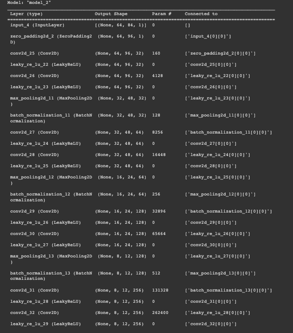
model.summary() should look similar to below:

Training
I encourage you to play with different optimizers and hyperparameters because it is exciting how they affect model KPIs. I will leave you the template for testing SGD and Adam, so have fun!
optimizer1 = tf.optimizers.SGD(learning_rate=1E-2, momentum=0.9, nesterov=True)
optimizer2 = tf.optimizers.Adam()
model.compile(loss='categorical_crossentropy',
              optimizer=optimizer2,
              metrics=['accuracy'])
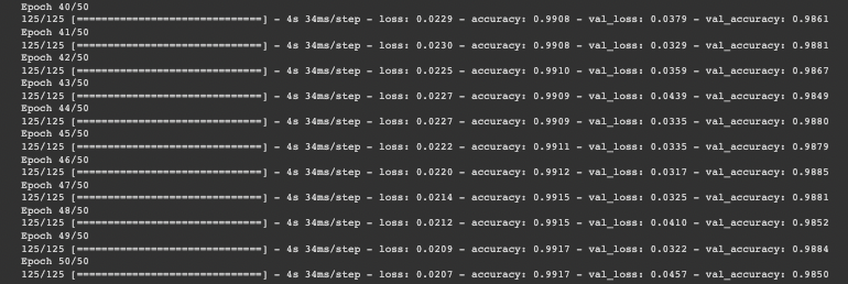
And we are ready to launch the training. Fifty epochs should be enough to get the appropriate accuracy.
EPOCHS = 50

steps_per_epoch = 4000//BATCH_SIZE
validation_steps = 800//BATCH_SIZE
test_steps = 200//BATCH_SIZE


history = model.fit(training_dataset,
                    steps_per_epoch=steps_per_epoch, validation_data=validation_dataset, validation_steps=validation_steps, epochs=EPOCHS)
By epoch 40, your validation accuracy should reach the 97% threshold.

Results
Let’s generate predictions for our dataset and calculate KPIs for our model. We aim to understand if it is ready to be deployed to production.
results = model.predict(test_dataset, steps=test_steps)results = np.argmax(results, axis=3)We will use two metrics:
- Intersection Over Union: area of overlap divided by area of union,
- Dice Score: area of overlap divided by the area of combination.
The basic idea is to measure how much our segmentation mask is the same as the label mask.
def class_wise_metrics(y_true, y_pred):
  '''
  Computes the class-wise IOU and Dice Score.

  Args:
    y_true (tensor) - ground truth label maps
    y_pred (tensor) - predicted label maps
  '''
  class_wise_iou = []
  class_wise_dice_score = []

  smoothing_factor = 0.00001

  for i in range(n_classes):
    intersection = np.sum((y_pred == i) * (y_true == i))
    y_true_area = np.sum((y_true == i))
    y_pred_area = np.sum((y_pred == i))
    combined_area = y_true_area + y_pred_area

    iou = (intersection) / (combined_area - intersection + smoothing_factor)
    class_wise_iou.append(iou)

    dice_score =  2 * ((intersection) / (combined_area + smoothing_factor))
    class_wise_dice_score.append(dice_score)

  return class_wise_iou, class_wise_dice_score
And we run the test. To make it fun, we add the slider and visualization so you can see different pictures.
# place a number here between 0 to 191 to pick an image from the test set
integer_slider = 150

ds = test_dataset.unbatch()
ds = ds.batch(200)
images = []

y_true_segments = []
for image, annotation in ds.take(2):
  y_true_segments = annotation
  images = image


iou, dice_score = class_wise_metrics(np.argmax(y_true_segments[integer_slider], axis=2), results[integer_slider])
show_annotation_and_prediction(image[integer_slider], annotation[integer_slider], results[integer_slider], iou, dice_score)
Now we can visualize the results. One on the left is the image. In the middle, you will see the label mask, and on the right, our prediction. Not bad, right?

Printing the results:
cls_wise_iou, cls_wise_dice_score = class_wise_metrics(np.argmax(y_true_segments, axis=3), results)

average_iou = 0.0
for idx, (iou, dice_score) in enumerate(zip(cls_wise_iou[:-1], cls_wise_dice_score[:-1])):
  print("Digit {}: IOU: {} Dice Score: {}".format(idx, iou, dice_score))
  average_iou += iou

grade = average_iou * 10

print("\nGrade is " + str(grade))
Our KPIs are pretty decent. You should see something similar to these numbers:

Model deployment
The deployment starts by saving the model and pushing it to the Model Registry. This special repository stores all model artifacts and manages versioning and access policies. I will cover the model registry when talking about AWS Sage Maker and Google Vertex, so now we will simply save the model and deploy it to the S3 bucket. You will be surprised to discover how many production systems use S3 buckets as their model repository and versioning system.
Save model in TF format – ‘.h5’. I would recommend using ‘.h5’ over pickle as later will not save object structure which is very important for the model. Almost always, it is better to save in ‘.h5’ over ‘.pkl’.
model.save("model.h5")We will talk about the S3 bucket in a moment. But first, we will create a simple server with REST API.
#import system libraries to work with filesystem and json
import os
import json
from json import dumps

#import to define input parameters type
from pydantic import BaseModel

#FastAPI will create us a nice and fast little server
from fastapi import FastAPI, UploadFile, File, HTTPException
from fastapi.middleware.cors import CORSMiddleware
from uvicorn import run

#import machine learning libraries
from tensorflow.keras.models import load_model
from tensorflow import expand_dims, cast, reshape, float32, int32
import numpy
from numpy import argmax
from numpy import max
from numpy import array
import pandas

#initiate server
app = FastAPI()

#man age CORS problem
origins = ["*"]
methods = ["*"]
headers = ["*"]

app.add_middleware(
    CORSMiddleware,
    allow_origins = origins,
    allow_credentials = True,
    allow_methods = methods,
    allow_headers = headers
)

#define input parameters
class Item(BaseModel):
    image: str

#lod model
model_dir = "model.h5"
model = load_model(model_dir)

@app.get("/")
def root():
    return {"message": "Welcome to the Semantic Segmentation API!"}

#add endpoint
@app.post("/net/image/segmentation/")
# def get_segmented_image(image_link: str = ""):
def get_segmented_image(image_data: Item):
    #if you want you can add further check of inputs
    # if image_data <check if image data exists and not empty>:
    #     raise HTTPException(status_code=415, detail="No image link provided")

    #load image from request body
    image_decoded = json.loads(image_data.image)
    image_numpy = numpy.array(image_decoded)

    #cast and preprocess image for model
    image = cast(image_numpy, dtype=float32)
    image = reshape(image, (image.shape[0], image.shape[1], 1))
    image = expand_dims(image, 0)
    image = image / 127.5
    image -= 1

    #generate presition
    prediction = model.predict(image)
    annotation = prediction = model.predict(image)

    #return segmentation map
    return {"respond": json.dumps(annotation.tolist())}

#our server will run on port 5000
if __name__ == "__main__":
    port = int(os.environ.get('PORT', 5000))
    run(app, host="0.0.0.0", port=port)
Continue to the next part – Production ML: Deploying model to Virtual Machine. Part 3.

