This is the third part of the article. Please find the second part here – Production ML: Deploying model to Virtual Machine. Part 2.
Infrastructure
Now we need a cozy place for our server. You can use any infrastructure provider you like. For this article, I use AWS, but it does not mean you have to use it.
One helpful thing that I would encourage you to use, though, is the AWS Toolkit plugin for Visual Studio. And if you are not using Visual Studio, you know what to do.
Go to Plugins -> Search and type ‘AWS’. It usually appears first. Click install and wait until the installation completes. Documentation will help you set up and access your AWS account (I assume you have one, if not, please register).
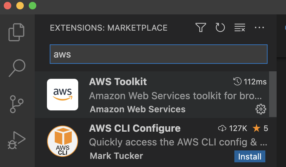
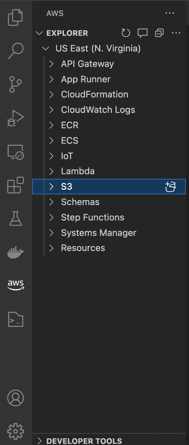
Once you are done, you should see the AWS section with some of your resources:
Compute
We will launch the EC2 instance now. Go to your AWS console and find the EC2 service console section.
AWS is changing the UI quite often, I find. So by the time you read, chances are something has changed. Please follow the logic and try to find the option I am referring to using common sense.
On the EC2 dashboard page, hit the big colorful button on the right and choose ‘Launch instances’.
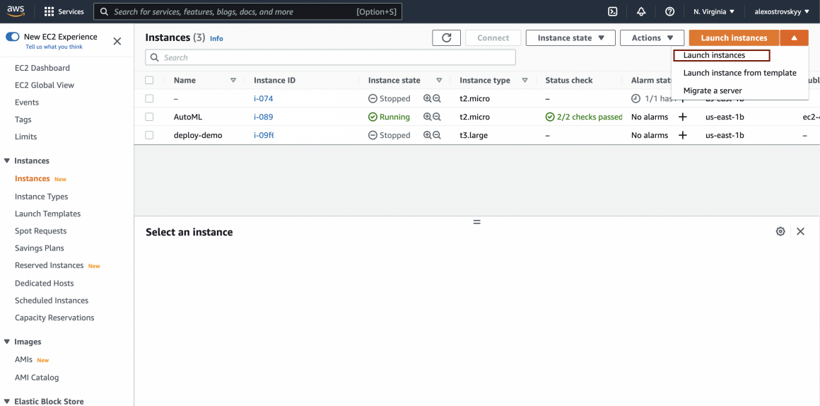
Name your instance and click on the ‘Browse more AMIs’ link.
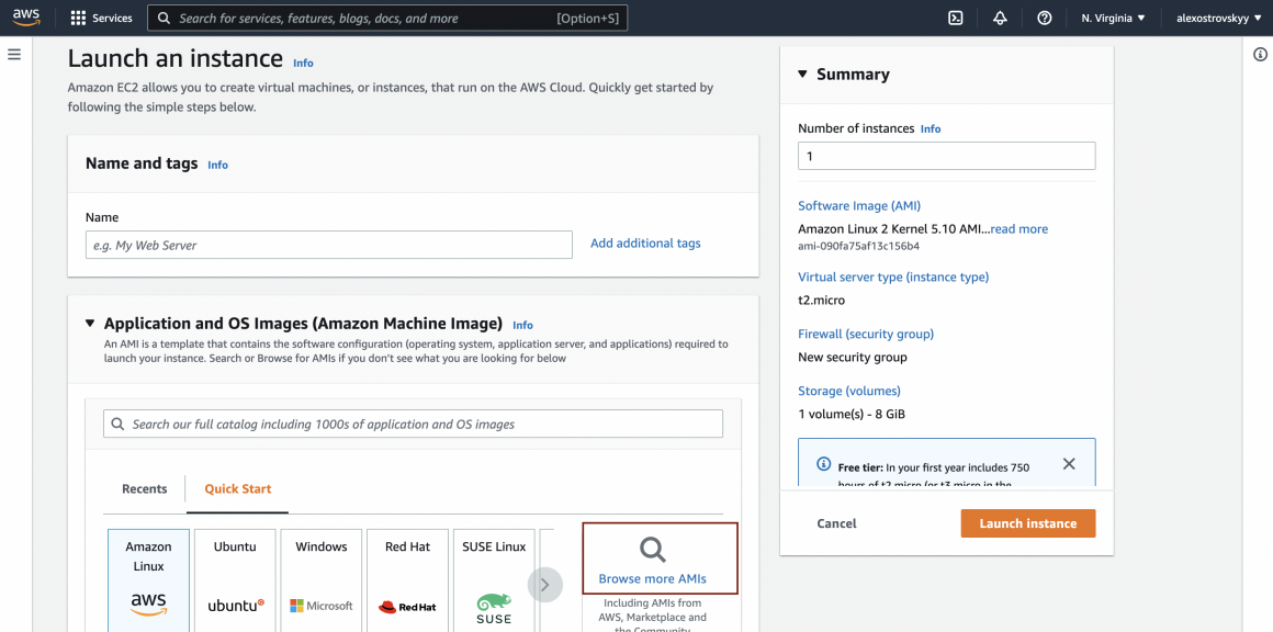
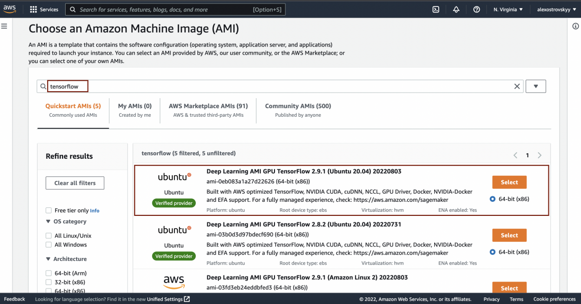
Type ‘TensorFlow’ in the search bar, and you will see a few Deep Learning optimized images. We will use these to avoid installing essential software on our own. Please pay attention to the versions of TF installed on the AMI. Ideally, it should be close to what you used when training the model.
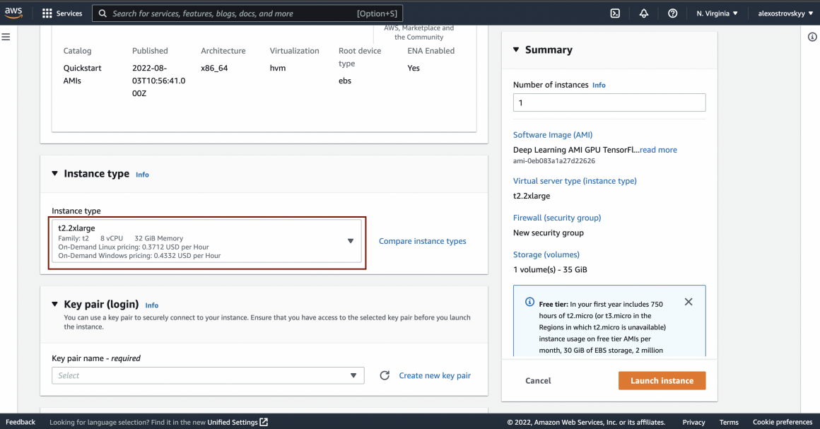
Now you can choose your instance type. I would recommend t2.2xlarge; it worked well for me. But you can try other instances and see how instance parameters affect the results. You can change the instance type later, but this would require the instance to be stopped.
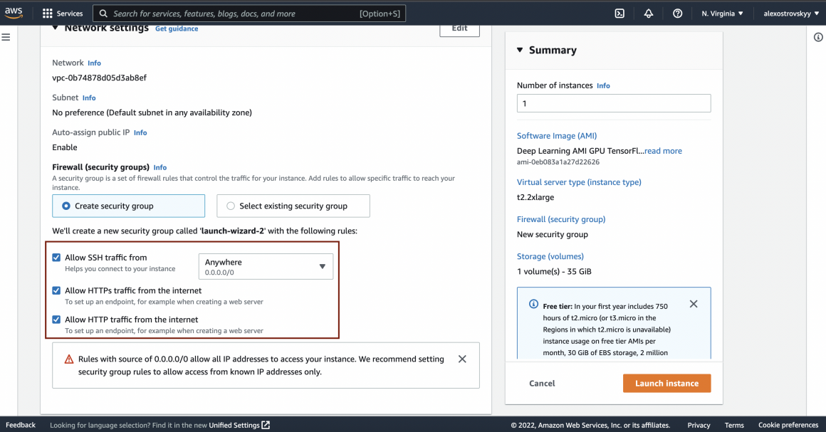
Next, let’s allow traffic to the instance:
And click ‘Launch instance’:
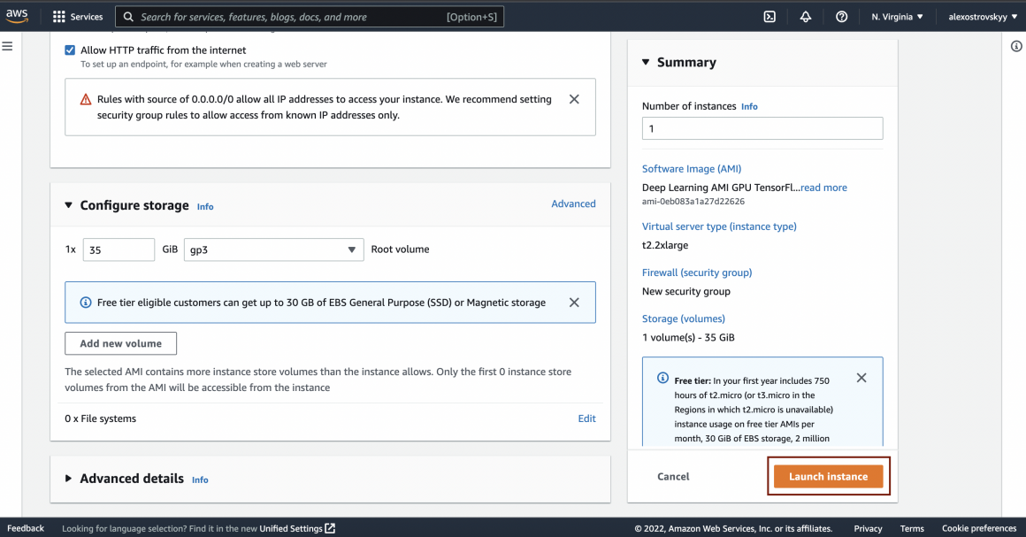
The instance will appear on the list of your instances. Not bad, right?
S3 Bucket
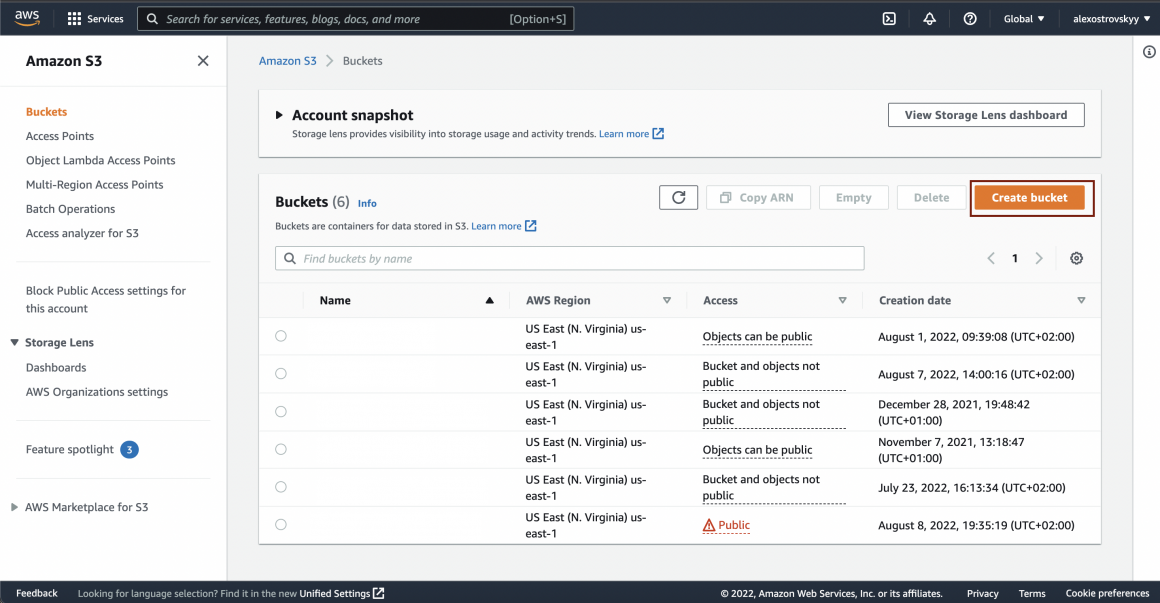
You can type S3 in AWS consol search bar and go to S3 daschboard.
There it is very simple to create a new bucket:
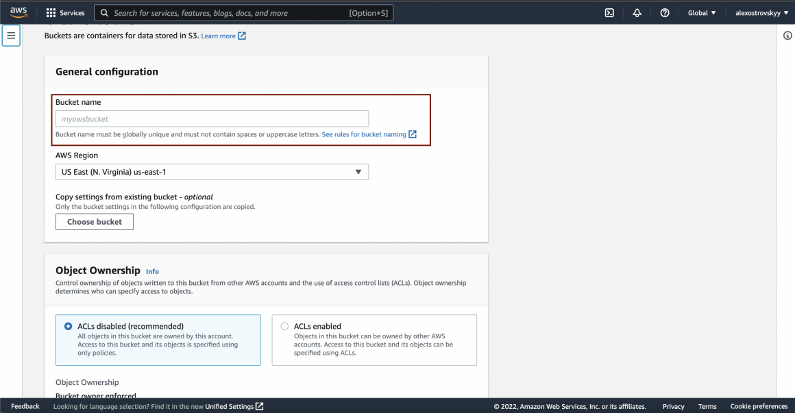
Type a sounding name for your bucket and click ‘Create’:
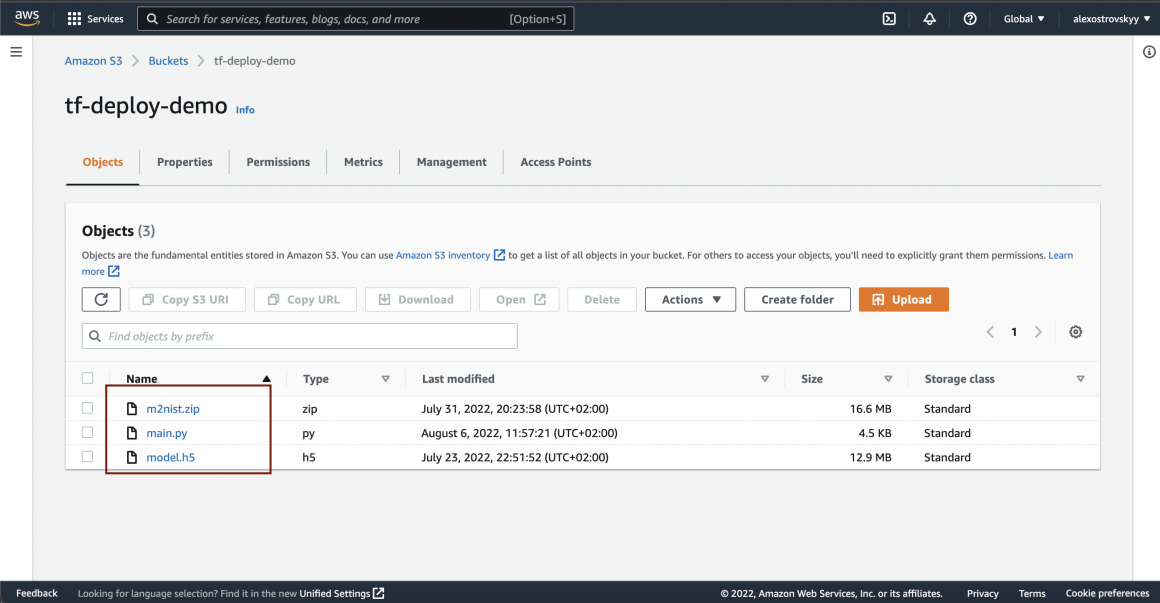
Once the bucket is up and running, you can upload your model and server script there:
IAM role
The VM we created earlier will have access to the bucket. It needs access to pull the latest version of our model and server script before starting the server.
For the EC2 instance to access our non-public bucket, we have to provide it with permission. To do that, we will create a new role that the instance will use.
Find the IAM dashboard in your AWS console and go to the Roles section:
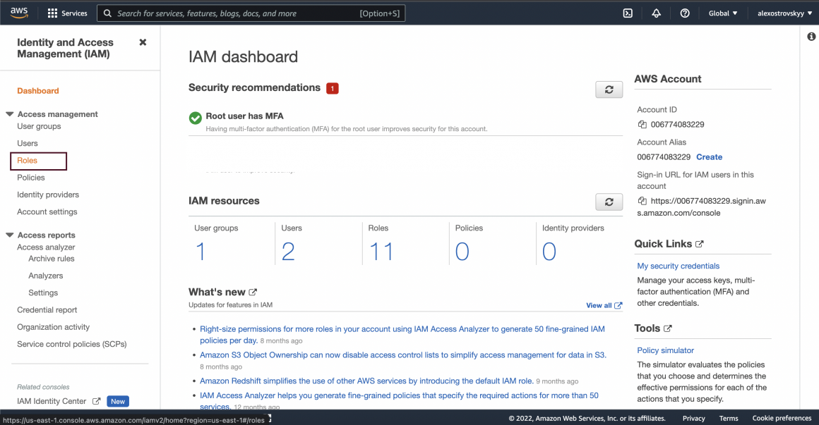
Start new role creation flow:
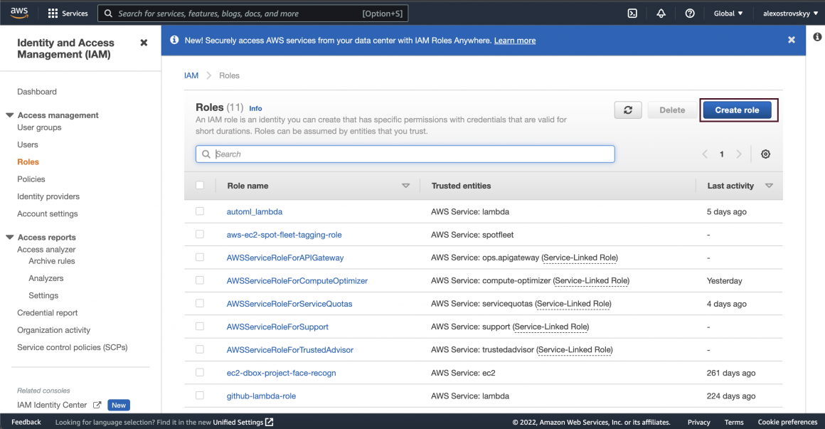
Choose AWS service -> EC2 as trusted entity type:
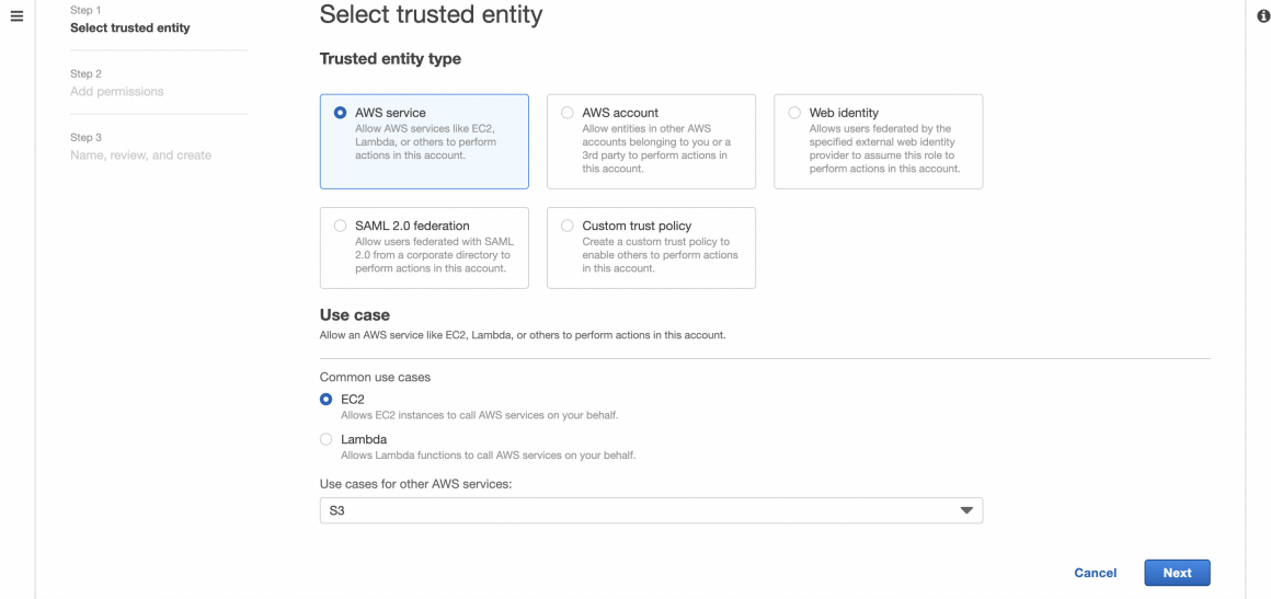
Click next and name your role:
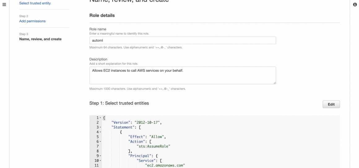
On the next screen, you will assign the required permission policy. We will simply provide our instance with full access to S3. In a production environment, this is not recommended. You will have to give specific and granular access to the particular bucket.
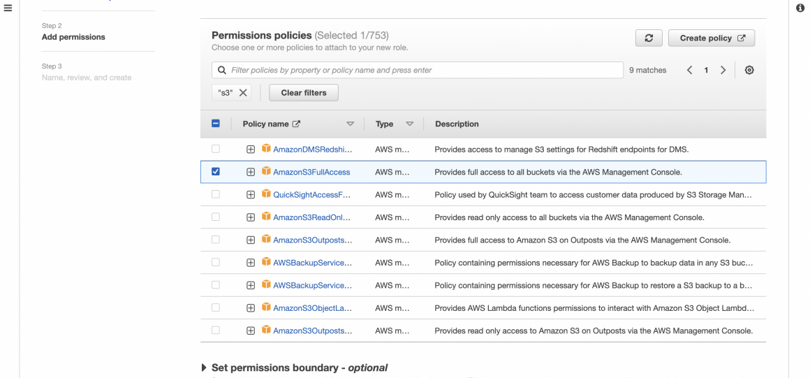
Now you can create the role.
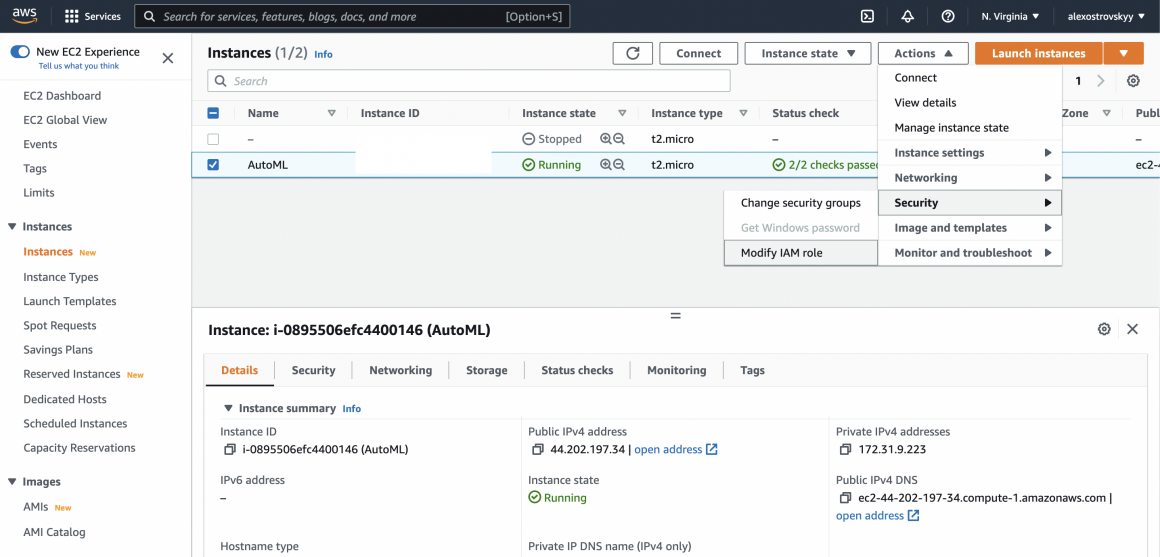
And assign a new role to the EC2 instance. To do that, you can go back to the EC2 dashboard, choose your instance and click the ‘Actions’ menu. Then go to the Security section of it and click ‘Modify IAM role’.
Launch the server
Everything is ready, and we can launch our server.
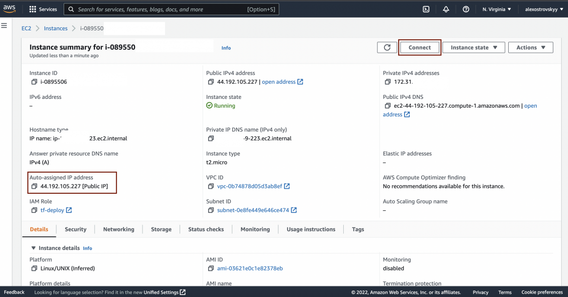
Click on the instance name, and you will see the instance summary. Note your instance external IP, and you will need it later when sending the API request. Click ‘Connect’ and open the instance connection section.
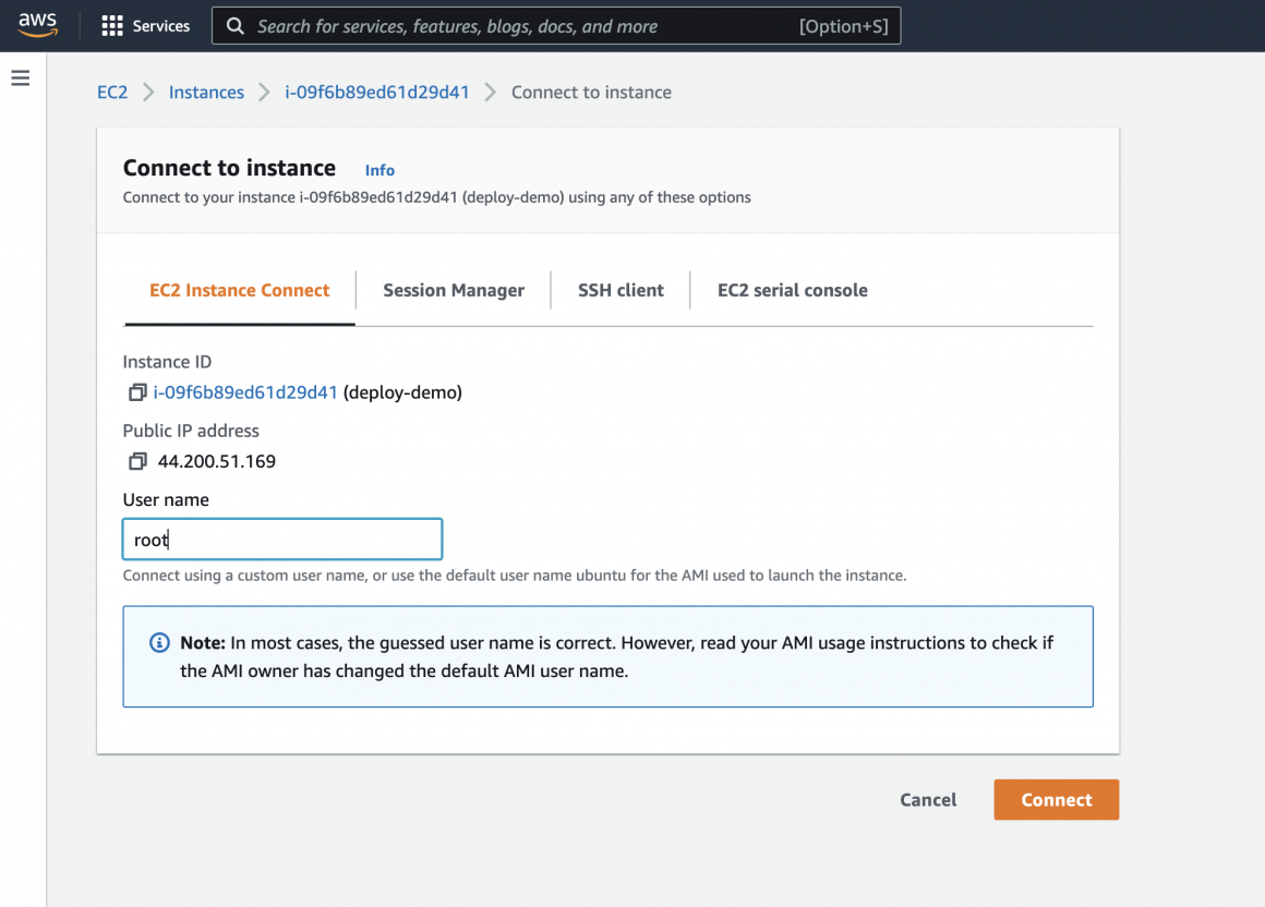
On the connection screen, type ‘root’ in username and click the ‘Connect’ button. If necessary, it will be easier for you to install all additional packages from the ‘root’ user.
Now you should see the following connection screen:
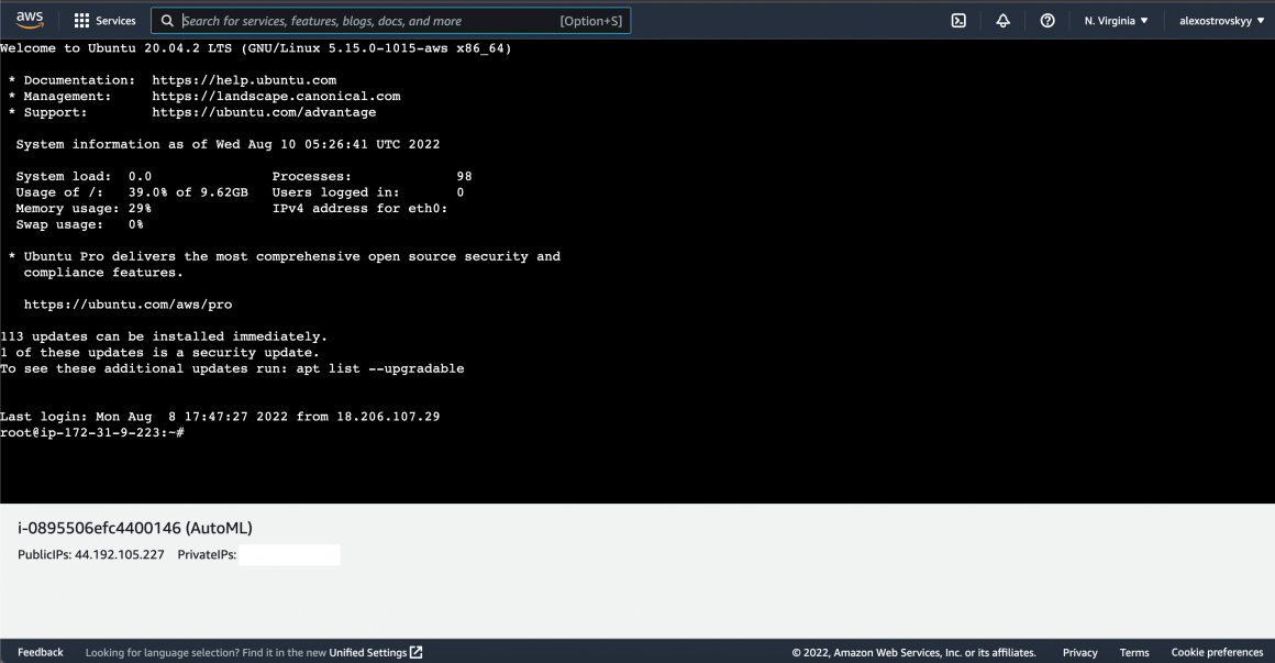
In an ideal scenario, you will only have to install AWS CLI on your EC2 instance. To do that type:
apt install awscli
This command will pull everything from your bucket to the VM disk. If you execute it again, it will only pull the file that had been changed, which can be helpful if you edit the file in your bucket using the Visual Studio AWS plugin. Once done, you can access your bucket from CLI on the EC2.

If you have trouble pulling the contents of your bucket, it can be either problem with:
- the role, or with
- region of your bucket,
- or with the network set-up of your VM.
You can return to the part where we spin up the VM, create a role for it, and ensure you did everything right. If that is not a cause of a problem, then you should also check if your bucket is in the same region as your VM. This can be checked in the Property tab of the S3 bucket and the Networking tab of the EC2 instance.
The version of Tensorflow in AWS MI may be outdated and not have pandas. This is one of the complications when you have to deal with VM and not the container. In such a case, it is best if you
- install conda to the VM,
- create a separate conda environment,
- activate conda env,
- install required Tensorflow version,
- install NumPy and pandas,
- restart VM,
- connect to VM, activate the conda env you created, and try again.
Hopefully, that will resolve the issue, so now you can
Test API
Now everything is working, and we can test our model live. You can go back to the colab environment and use the following code:
#import some libraries
import numpy
import tensorflow
from tensorflow.keras.models import load_model
from tensorflow import expand_dims, cast, reshape, float32, int32

import requests
import json

import pprint
import PIL.Image, PIL.ImageFont, PIL.ImageDraw
from matplotlib import pyplot as plt

images_depl = numpy.load('/tmp/training/combined.npy')
I usually prefer pulling the dataset from my gdrive because I will not have to upload it every time I restart the kernel manually.
from google.colab import drive
drive.mount('/content/gdrive')
Let’s take any image:
demo_dump = json.dumps(images_depl[3].tolist())And send it to our server. Please do not forget to put your server’s external IP in the code below:
headers = {"content-type": "application/json"}
demo_json = {'image' : demo_dump}
json_response = requests.post('http://<your_ec2_server_ip>:5000/net/image/segmentation/', json=demo_json, headers=headers)
Read the response:
responce_server = json.loads(json.loads(json_response.text)['respond'])
responce_server_numpy = numpy.array(responce_server)
With the help of these functions, we will be able to visualize the prediction of our server:
# there are 11 classes in the dataset: one class for each digit (0 to 9) plus the background class
n_classes = 11

# assign a random color for each class
colors = [tuple(numpy.random.randint(256, size=3) / 255.0) for i in range(n_classes)]

def give_color_to_annotation(annotation):
  '''
  Converts a 2-D annotation to a numpy array with shape (height, width, 3) where
  the third axis represents the color channel. The label values are multiplied by
  255 and placed in this axis to give color to the annotation

  Args:
    annotation (numpy array) - label map array

  Returns:
    the annotation array with an additional color channel/axis
  '''
  seg_img = numpy.zeros( (annotation.shape[0],annotation.shape[1], 3) ).astype('float')

  for c in range(n_classes):
    segc = (annotation == c)
    seg_img[:,:,0] += segc*( colors[c][0] * 255.0)
    seg_img[:,:,1] += segc*( colors[c][1] * 255.0)
    seg_img[:,:,2] += segc*( colors[c][2] * 255.0)

  return seg_img

def show_annotation_and_image(image, annotation):
  '''
  Displays the image and its annotation side by side

  Args:
    image (numpy array) -- the input image
    annotation (numpy array) -- the label map
  '''
  # new_ann = numpy.argmax(annotation, axis=2)
  seg_img = give_color_to_annotation(annotation[0])
  image = image + 1
  image = image * 127.5
  image = numpy.reshape(image, (image.shape[1], image.shape[2],))

  image = numpy.uint8(image)
  images = [image, seg_img]

  images = [image, seg_img]
  fused_img = fuse_with_pil(images)
  plt.imshow(fused_img)

def fuse_with_pil(images):
  '''
  Creates a blank image and pastes input images

  Args:
    images (list of numpy arrays) - numpy array representations of the images to paste

  Returns:
    PIL Image object containing the images
  '''

  widths = (image.shape[1] for image in images)
  heights = (image.shape[0] for image in images)
  total_width = sum(widths)
  max_height = max(heights)

  new_im = PIL.Image.new('RGB', (total_width, max_height))

  x_offset = 0
  for im in images:
    pil_image = PIL.Image.fromarray(numpy.uint8(im))
    new_im.paste(pil_image, (x_offset,0))
    x_offset += im.shape[1]

  return new_im
And here we go, our prediction:
show_annotation_and_image(image, results_final)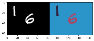
Conclusion
This was a long article—actually long few articles. And I am sincerely grateful to you who read it all and did everything together with me.
Now you know how to deploy your model to a VM and serve the prediction. You can now spin up a scale set, create a simple deployment script that will install AWS CLI and pull necessary files, and have a scalable production solution. Which is not bad, right?
Or you can follow me to the next step of our journey, where we explore the power of containers and serverless cloud services.
See you in the following article!


