In previous articles, we’ve learned how to ingest the data from our data lake, analyze and balance our data, and run production-grade feature engineering on AWS. Today, we will talk about model training and deployment.
This is not the last article in this series. Next, we will discuss model monitoring, automated retraining, and explainability. So, stay tuned!
Prerequisites
First, you must choose the environment where you will run your automated pipeline. This environment will be an orchestrator, launching training, testing, and deployment jobs. It doesn’t have to be too large. Depending on the configuration of the jobs in your pipeline, it will take 40 minutes to a couple of hours to run your pipeline, so stability is a more critical factor. For this reason, I would not recommend using the free version of Colab, for example.
I will be using Sagemaker Studio Notebooks. If you want to use it also, please read the first article of the series (Private: Production ML: Training and deploying model with AWS AutoML, SageMaker, Glue, and Athena. Part 1.), which will explain how to configure your Studio.
Let us begin our party then by installing the Sagemaker in our env:
!pip install -U sagemaker -qI assume you are using Data Science images with many useful tools installed and available. Therefore I will import them. If this is not the case, you know what to do ;).
import pandas as pd
import numpy as np
import matplotlib.pyplot as plt
from time import gmtime, strftime, sleep
from pprint import pprint
import json
import io
from urllib.parse import urlparse
from sklearn.metrics import (
    roc_auc_score,
    roc_curve,
    precision_recall_curve,
    classification_report,
    average_precision_score,
    precision_score,
    recall_score,
)
import matplotlib.pyplot as plt
My account has a Batch Transform limit of four for ml.m5.xlarge instances in my account, impacting how many candidate models from the list of ten candidates I will use to test the models. I will only take the four best models trained by AutoML and check their precision, recall, and f1-score on the test dataset.
TOP_N_CANDIDATES = 4Next, we will initialize Sagemaker session.
import sagemaker
from sagemaker import AutoML
import boto3
from sagemaker import get_execution_role

print(sagemaker.__version__)

region = boto3.Session().region_name

session = sagemaker.Session()

# You can modify the following to use a bucket of your choosing
bucket = session.default_bucket()
prefix = "<your-bucket-name>"

role = get_execution_role()

sm = boto3.Session().client(service_name="sagemaker", region_name=region)
The session will take care of many things, including S3 buckets, data allocation and movement, roles, statuses and descriptions of jobs, etc.
Dataset
We will use the dataset describing customer churn for one of the telecom providers. It is relatively small in size (only 5000 records) and contains 21 user attributes:
State: the US state in which the customer resides, indicated by a two-letter abbreviation; for example, OH or NJAccount Length: the number of days that this account has been activeArea Code: the three-digit area code of the corresponding customer’s phone numberPhone: the remaining seven-digit phone numberInt’l Plan: whether the customer has an international calling plan: yes/noVMail Plan: whether the customer has a voice mail feature: yes/noVMail Message: presumably the average number of voice mail messages per monthDay Mins: the total number of calling minutes used during the dayDay Calls: the total number of calls placed during the dayDay Charge: the billed cost of daytime callsEve Mins, Eve Calls, Eve Charge: the billed cost for calls placed during the eveningNight Mins,Night Calls,Night Charge: the billed cost for calls placed during nighttimeIntl Mins,Intl Calls,Intl Charge: the billed cost for international callsCustServ Calls: the number of calls placed to Customer ServiceChurn?: whether the customer left the service: true/false
As you probably guessed from the attributes’ description, we will train our models to predict Churn.
The previous article described the data validation and preparation process in automated production pipelines with AWS Athena, Data Wrangler, and Sagemaker Clarify. Alternatively, you can use, for example, PyDeequ, a Python API for the Deequ – library, which will help you validate massive datasets and build on top of Apache Spark. Therefore we will not cover the initial steps of our production pipeline and focus on the training and deployment.
You can download dataset here:
And read it from the file:
churn = pd.read_csv("./churn.txt")
churn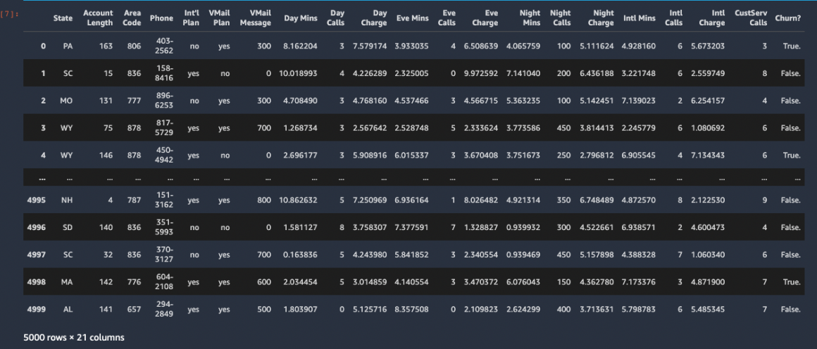
Let’s divide our data to train and test datasets:
train_data = churn.sample(frac=0.8, random_state=200)

test_data = churn.drop(train_data.index)

test_data_no_target = test_data.drop(columns=["Churn?"])
And save them in CSV format:
train_file = "train_data.csv"
train_data.to_csv(train_file, index=False, header=True)

test_file = "test_data.csv"
test_data_no_target.to_csv(test_file, index=False, header=False)
Training
So far, everything in this article has been easy. In my experience with AutoML pipelines (AWS, Google, Azure, H2O), data validation and quality management are the most difficult parts.
The next section describes everything we need to start the model training:
timestamp_suffix = strftime("%d-%H-%M-%S", gmtime())
base_job_name = "automl-churn-sdk-" + timestamp_suffix

target_attribute_name = "Churn?"
target_attribute_values = np.unique(train_data[target_attribute_name])
target_attribute_true_value = target_attribute_values[1]  # 'True.'

#configure AutoML jobs
automl = AutoML(
    role=role,
    target_attribute_name=target_attribute_name,
    base_job_name=base_job_name,
    sagemaker_session=session,
    max_candidates=10,
)
This line will start the configured AutoML training jobs with our train dataset.
automl.fit(train_file, job_name=base_job_name, wait=False, logs=False)You can monitor job status with following code:
print("JobStatus - Secondary Status")
print("------------------------------")


describe_response = automl.describe_auto_ml_job()
print(describe_response["AutoMLJobStatus"] + " - " + describe_response["AutoMLJobSecondaryStatus"])
job_run_status = describe_response["AutoMLJobStatus"]

while job_run_status not in ("Failed", "Completed", "Stopped"):
    describe_response = automl.describe_auto_ml_job()
    job_run_status = describe_response["AutoMLJobStatus"]

    print(
        describe_response["AutoMLJobStatus"] + " - " + describe_response["AutoMLJobSecondaryStatus"]
    )
    sleep(100)
The loop will print the status every 100 seconds:
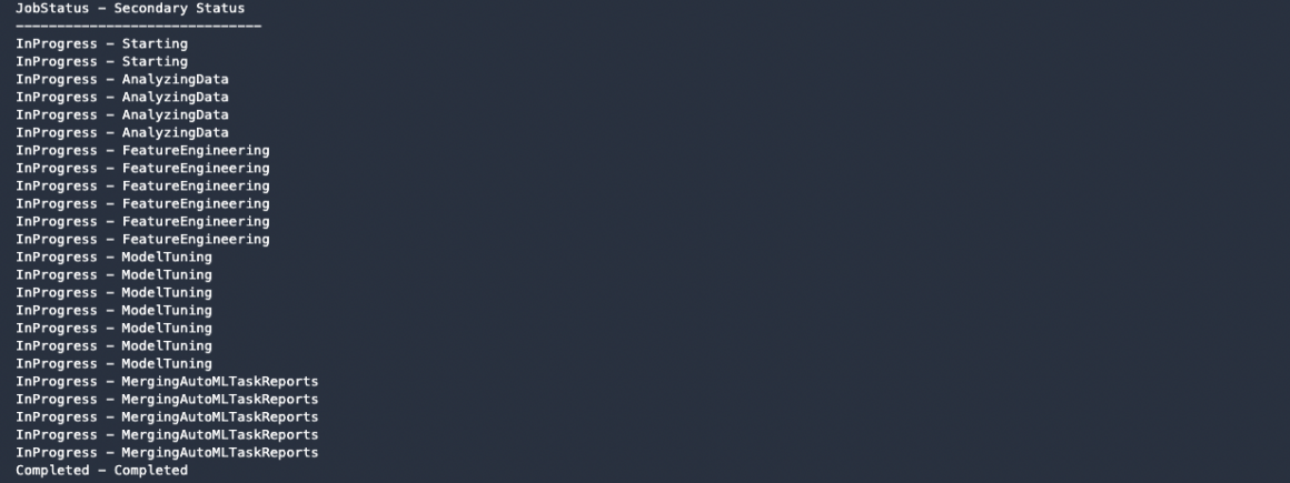
When training is completed, we can deploy the model or explore the list of candidates to find the best one based on our specific needs.
Candidates
Let’s list the top four candidates we will be assessing:
candidates = automl.list_candidates(
    sort_by="FinalObjectiveMetricValue", sort_order="Descending", max_results=TOP_N_CANDIDATES
)

for candidate in candidates:
    print("Candidate name: ", candidate["CandidateName"])
    print("Objective metric name: ", candidate["FinalAutoMLJobObjectiveMetric"]["MetricName"])
    print("Objective metric value: ", candidate["FinalAutoMLJobObjectiveMetric"]["Value"])
    print("\n")
The list of validation metrics (f1) values for top four models:

We can pull the best-performer model usingdescribe_auto_ml_job() method:
best_candidate = automl.describe_auto_ml_job()["BestCandidate"]
best_candidate_name = best_candidate["CandidateName"]
print("CandidateName: " + best_candidate_name)
print(
    "FinalAutoMLJobObjectiveMetricName: "
    + best_candidate["FinalAutoMLJobObjectiveMetric"]["MetricName"]
)
print(
    "FinalAutoMLJobObjectiveMetricValue: "
    + str(best_candidate["FinalAutoMLJobObjectiveMetric"]["Value"])
)
Testing
Now we will use our test dataset to test the performance of the four best models.
First of all, let’s upload the test dataset to the S3 bucket:
input_data_transform = session.upload_data(path=test_file, bucket=bucket, key_prefix=prefix)And configure the Sagemaker Autopilot inference containers. In binary and multiclass classification, inference containers can produce label(s) and probability(es) for the label(s). In our case (binary classification), we will have only one label and probability, and we will ask the model to tell us both values:
inference_response_keys = ["predicted_label", "probability"]

s3_transform_output_path = "s3://{}/{}/inference-results/".format(bucket, prefix)

transformers = []

for candidate in candidates:
    model = automl.create_model(
        name=candidate["CandidateName"],
        candidate=candidate,
        inference_response_keys=inference_response_keys,
    )

    output_path = s3_transform_output_path + candidate["CandidateName"] + "/"

    transformers.append(
        model.transformer(
            instance_count=1,
            instance_type="ml.m5.xlarge",
            assemble_with="Line",
            output_path=output_path,
        )
    )
Now we can run the transform jobs:
for transformer in transformers:
    transformer.transform(
        data=input_data_transform, split_type="Line", content_type="text/csv", wait=False
    )
    print("Starting transform job {}".format(transformer._current_job_name))
pending_complete = True

while pending_complete:
    pending_complete = False
    num_transform_jobs = len(transformers)
    for transformer in transformers:
        desc = sm.describe_transform_job(TransformJobName=transformer._current_job_name)
        if desc["TransformJobStatus"] not in ["Failed", "Completed"]:
            pending_complete = True
        else:
            num_transform_jobs -= 1
    print("{} out of {} transform jobs are running.".format(num_transform_jobs, len(transformers)))
    sleep(100)

for transformer in transformers:
    desc = sm.describe_transform_job(TransformJobName=transformer._current_job_name)
    print(
        "Transform job '{}' finished with status {}".format(
            transformer._current_job_name, desc["TransformJobStatus"]
        )
    )
You will soon see that your transform jobs have been finished. Ideally, it should happen with the status “Completed”:

Here is a short function we will use to gather the inference results of our candidates:
def get_csv_from_s3(s3uri, file_name):
    parsed_url = urlparse(s3uri)
    bucket_name = parsed_url.netloc
    prefix = parsed_url.path[1:].strip("/")
    s3 = boto3.resource("s3")
    obj = s3.Object(bucket_name, "{}/{}".format(prefix, file_name))
    return obj.get()["Body"].read().decode("utf-8")
Let’s read the results produced by top four candidates:
predictions = []

for transformer in transformers:
    print(transformer.output_path)
    pred_csv = get_csv_from_s3(transformer.output_path, "{}.out".format(test_file))
    predictions.append(pd.read_csv(io.StringIO(pred_csv), header=None))
And analyse the outcomes:
labels = test_data[target_attribute_name].apply(
    lambda row: True if row == target_attribute_true_value else False
)

# calculate auc score
for prediction, candidate in zip(predictions, candidates):
    roc_auc = roc_auc_score(labels, prediction.loc[:, 1])
    ap = average_precision_score(labels, prediction.loc[:, 1])
    print(
        "%s's ROC AUC = %.2f, Average Precision = %.2f" % (candidate["CandidateName"], roc_auc, ap)
    )
    print(classification_report(test_data[target_attribute_name], prediction.loc[:, 0]))
    print()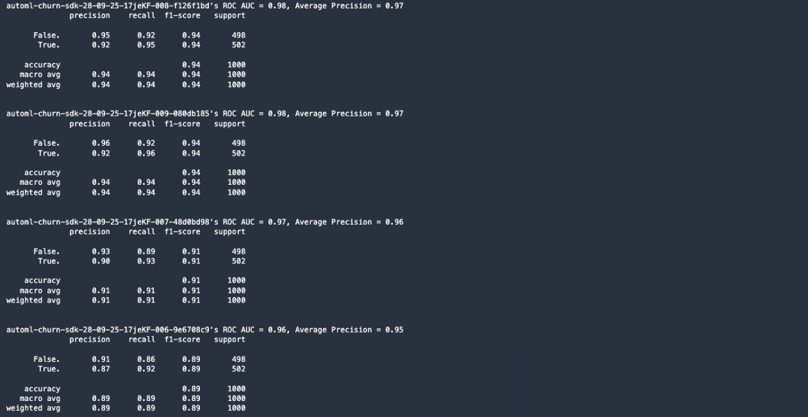
If you want you can plot ROC and Precision-Recall curves, like so:
fpr_tpr = []
for prediction in predictions:
    fpr, tpr, _ = roc_curve(labels, prediction.loc[:, 1])
    fpr_tpr.append(fpr)
    fpr_tpr.append(tpr)

plt.figure(num=None, figsize=(16, 9), dpi=160, facecolor="w", edgecolor="k")
plt.plot(*fpr_tpr)
plt.legend([candidate["CandidateName"] for candidate in candidates], loc="lower right")
plt.xlabel("False Positive Rate")
plt.ylabel("True Positive Rate")
plt.title("ROC Curve")
plt.show()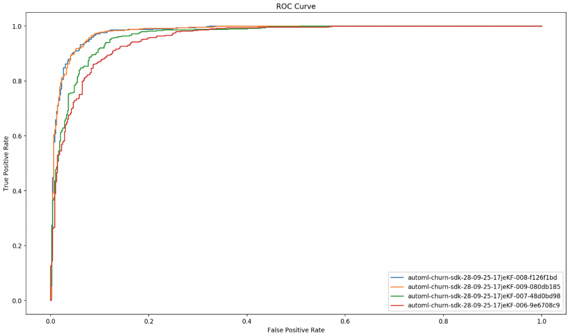
precision_recall = []
for prediction in predictions:
    precision, recall, _ = precision_recall_curve(labels, prediction.loc[:, 1])
    precision_recall.append(recall)
    precision_recall.append(precision)

plt.figure(num=None, figsize=(16, 9), dpi=160, facecolor="w", edgecolor="k")
plt.plot(*precision_recall)
plt.legend([candidate["CandidateName"] for candidate in candidates], loc="lower left")
plt.xlabel("Recall")
plt.ylabel("Precision")
plt.title("Precision-Recall Curve")
plt.show()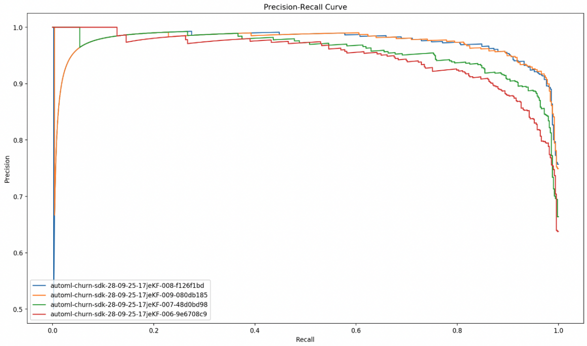
As I mentioned, you can choose the model with the best f1 score and deploy it to the endpoint. But in some cases, precision might have more weight over the recall or vice versa. For example, we sometimes can decide to value recall over precision in this situation. This can happen because we want to target all people in the risk zone, even if that means that sometimes people who are not in the risk group will receive a reactivation incentive.
In such cases, we can lower our expectations in precision space to gain recall accuracy. I assume you know why these two have a negative correlation. Let’s imagine we are ok to lower the precision accuracy expectation to achieve better recall accuracy.
target_min_precision = 0.75

best_recall = 0
best_candidate_idx = -1
best_candidate_threshold = -1
candidate_idx = 0
for prediction in predictions:
    precision, recall, thresholds = precision_recall_curve(labels, prediction.loc[:, 1])
    threshold_idx = np.argmax(precision >= target_min_precision)
    if recall[threshold_idx] > best_recall:
        best_recall = recall[threshold_idx]
        best_candidate_threshold = thresholds[threshold_idx]
        best_candidate_idx = candidate_idx
    candidate_idx += 1

print("Best Candidate Name: {}".format(candidates[best_candidate_idx]["CandidateName"]))
print("Best Candidate Threshold (Operation Point): {}".format(best_candidate_threshold))
print("Best Candidate Recall: {}".format(best_recall))
In such a case, we can update the operation point to give us 100% recall accuracy on the test dataset.
prediction_default = predictions[best_candidate_idx].loc[:, 0] == target_attribute_true_value
prediction_updated = predictions[best_candidate_idx].loc[:, 1] >= best_candidate_threshold

print(
    "Default Operating Point: recall={}, precision={}".format(
        recall_score(labels, prediction_default), precision_score(labels, prediction_default)
    )
)
print(
    "Updated Operating Point: recall={}, precision={}".format(
        recall_score(labels, prediction_updated), precision_score(labels, prediction_updated)
    )
)
Deployment
At this stage, we will configure and call the model deployment method like so:
from sagemaker.predictor import Predictor
from sagemaker.serializers import CSVSerializer
from sagemaker.deserializers import CSVDeserializer

predictor = automl.deploy(
    initial_instance_count=1,
    instance_type="ml.m5.2xlarge",
    candidate=candidates[best_candidate_idx],#best_candidate if you did not update the operating point
    inference_response_keys=inference_response_keys,
    predictor_cls=Predictor,
    serializer=CSVSerializer(),
    deserializer=CSVDeserializer(),
)

print("Created endpoint: {}".format(predictor.endpoint_name))
When you run this code, you will see the name of the endpoint to which you’ve just deployed your model:

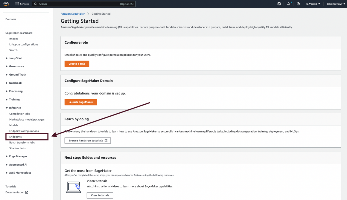
You will find it in your Sagemaker Studio in the “Endpoints’ section under the “Inference” section:
Summary
When the AutoML job is finished, you can check your Sagemaker S3 bucket to see all of the output artifacts:
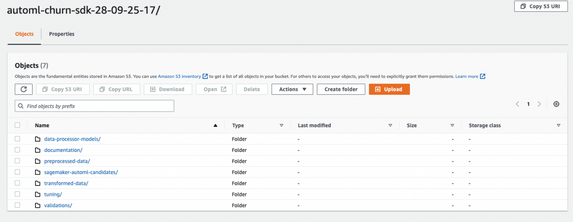
The folder ‘data-processor-models’ will contain model candidates. In ‘sagemaker-automl-candidates’, you will find the data processing code required to prepare the data for the training and train models.
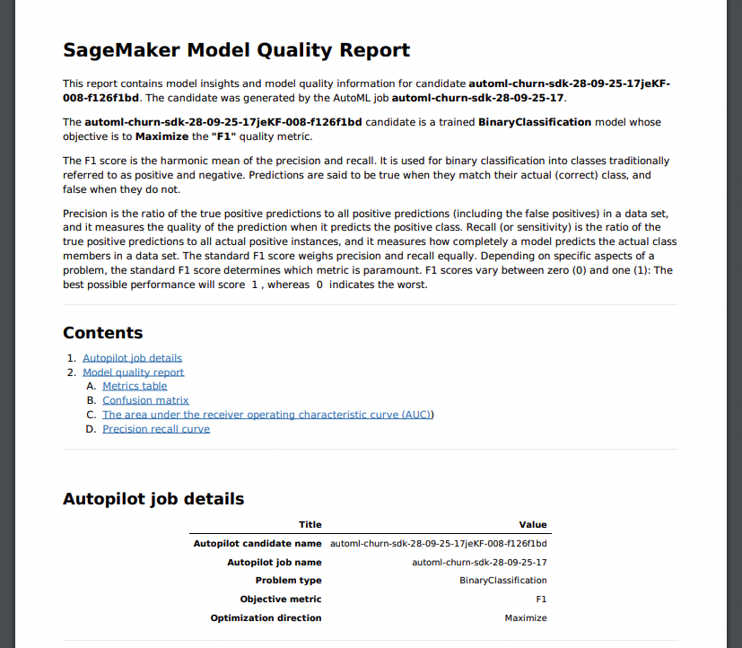
In the ‘documentation’ you will find model quality report (model_monitor subfolder):
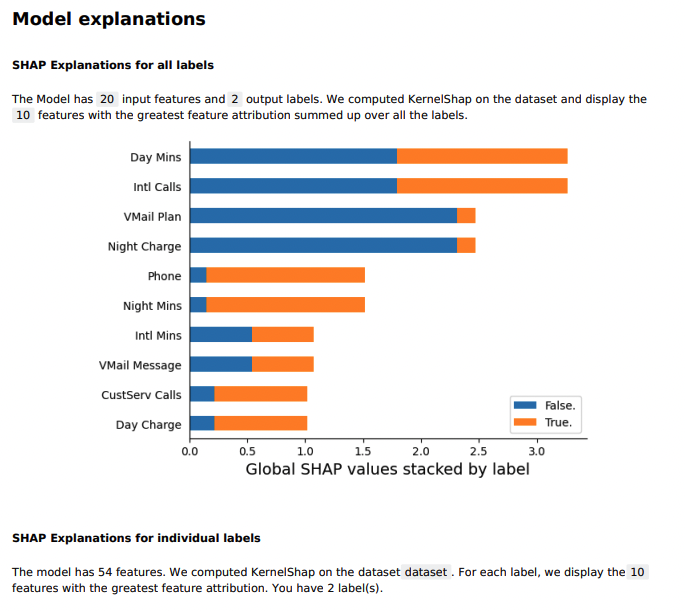
and feature importance report (explainability subfolder):
This article is longer than others, and I know I did not thoroughly explain every step and function. My task was to show you how easy it is to train and deploy great models using Sagemaker AutoML.
I would like you to take a look at the Sagemaker AutoML documentation. Their team did an excellent job designing, building, and documenting a state-of-the-art Machine Learning framework.
In one of the following articles, I will show you Google Cloud AutoML capabilities, a very simple, powerful, and elegant framework.
Stay tuned, and may the Force be with you!

