Data Ingestion and Validation in Production Machine Learning. Structured Dataset.

This article is a part of a series called “Production ML“.

Introduction

Today we will talk about data ingestion in Production Machine Learning systems. What makes it unique in production that we apply special tools and techniques? It’s a few things:

1. The amount of data is such that we will not be able to wrangle it on our laptop or one VM in the cloud. In production, data processing often requires a massive amount of computing power and splitting the workload between the compute nodes.
2. The dataset’s quality in real life is very different from the one we use to build PoC. It’s not clean, is often skewed, and contains corrupted datapoints.
3. When the system is working in production, it requires a continuous supply of data, training, validation, and deployment iterations. Therefore usually, we design and build an automated pipeline that assures the continuity of the process.
4. During data ingestion and transformation, training, deployment, and serving, we generate and store tons of metadata and historical information, which we will use later to investigate and improve.

First of all, we want our Pipeline to read the data. Then, define data statistics and Schema, which it will use to validate the data.

If Pipeline spots problems with data it should notify us so we can decide on what to do. Another option is to let Pipeline make decisions within certain boundaries. For example, we can instruct the Pipeline to add missing values to the Feature Domain or reduce the sensitivity for certain features.

For the demonstration, we will use Census Income Dataset. This Dataset is used to predict the income of individuals. In particular, a label defines if a person’s yearly earnings are less than 50k or more. The Features are:

• age;
• workclass;
• fnlwgt;
• education;
• education-num;
• marital-status;
• occupation;
• relationship;
• race;
• sex;
• capital-gain;
• capital-loss;
• hours-per-week;
• native-country.

We will investigate the possible values of the Features below. We chose this Dataset because it is easily accessible for you, so you will not have trouble reproducing the code from this and further articles. For production purposes, it is too clean, so we will have to make it less sterile and accurate.

So let’s start ramping up the data ingestion and validation part of our Production Pipeline. I recommend you follow me in Google colab; it is the easiest way to start fast. In the future, the calculations we make will be so efficient that for this Dataset, you don’t even need GPUs in colab.

Libraries

We will install TFX:

!pip install -U --quiet tfx

If you’re working in the colab, please restart your runtime. After the restart, we will have to import a few libraries:

import tensorflow as tf
print('TF: {}'.format(tf.__version__))

import tensorflow_data_validation as tfdv
print('TFDV: {}'.format(tfdv.__version__))

import pandas as pd
from sklearn.model_selection import train_test_split

import seaborn as sns
import matplotlib
import matplotlib.pyplot as plt

import os

I hope none of them is new to you:

• tensorflow – is ML framework,
• import tensorflow_data_validation as tfdv – is part of TFX library,
• pandas – library we use to work with data in many formats,
• sklearn – one of the most popular python Machine Learning libraries,
• seaborn and matplotlib – will help us plot charts and other graphical representation of our information,
• os – python library that helps manipulate filesystem.

Load data

Let us download the Dataset:

train = './adult.data'
test = './adult.test'

if not os.path.exists(train):
  !wget https://archive.ics.uci.edu/ml/machine-learning-databases/adult/adult.data
  !wget https://archive.ics.uci.edu/ml/machine-learning-databases/adult/adult.test

We add logic to prevent us from downloading files if they already exist.

We read our data to pandas dataframe format:

header_list = ['age', 'workclass', 'fnlwgt', 'education', 'education-num', 'marital-status', 'occupation', 
               'relationship', 'race', 'sex', 'capital-gain', 'capital-loss', 'hours-per-week', 'native-country', 'label']
df = pd.read_csv('./adult.data', names=header_list, skipinitialspace=True)

Next, we will use thetrain_test_split function from sklearn to split the dataframe into two parts: test and evaluation:

train_df, eval_df = train_test_split(df, test_size=0.2, shuffle=False)

We will use this split to demonstrate the data validation part of the Pipeline. We want evaluation data to be slightly different from train data. And we want Pipeline to spot the difference and explain it to us.

To introduce the corrupted data, we will add a few datapoints to the dataframe, like so:

def add_malformed_rows(df):
    rows = [
        {
            'age': 46, 
            'fnlwgt': 257473, 
            'education': 'Bachelors', 
            'education-num': 8,
            'marital-status': 'Married-civ-spouse', 
            'occupation': 'Plumber', 
            'relationship': 'Husband', 
            'race': 'Other', 
            'sex': 'Male',
            'capital-gain': 1000, 
            'capital-loss': 0, 
            'hours-per-week': 41, 
            'native-country': 'Australia',
            'label': '>50K'
        },
        {
            'age': 0, 
            'workclass': 'New workclass', 
            'fnlwgt': 257473, 
            'education': 'Masters', 
            'education-num': 8,
            'marital-status': 'Married-civ-spouse', 
            'occupation': 'Adm-clerical', 
            'relationship': 'Wife', 
            'race': 'Asian', 
            'sex': 'Female',
            'capital-gain': 0, 
            'capital-loss': 0, 
            'hours-per-week': 40, 
            'native-country': 'Pakistan',
            'label': '>50K'
        },
        {
            'age': 1000, 
            'workclass': 'Another new workclass', 
            'fnlwgt': 257473, 
            'education': 'Masters', 
            'education-num': 8,
            'marital-status': 'Married-civ-spouse', 
            'occupation': 'Prof-specialty', 
            'relationship': 'Husband', 
            'race': 'Black', 
            'sex': 'Male',
            'capital-gain': 0, 
            'capital-loss': 0, 
            'hours-per-week': 20, 
            'native-country': 'Cameroon',
            'label': '<=50K'
        },
        {
            'age': 25, 
            'workclass': 'Another new workclass', 
            'fnlwgt': 257473, 
            'education': 'Masters', 
            'education-num': 8,
            'marital-status': 'Married-civ-spouse', 
            'occupation': 'gamer', 
            'relationship': 'Husband', 
            'race': 'Asian', 
            'sex': 'Female',
            'capital-gain': 0, 
            'capital-loss': 0, 
            'hours-per-week': 50, 
            'native-country': 'Mongolia',
            'label': '<=50K'
        }
    ]
    
    df = df.append(rows, ignore_index=True)
    
    return df

eval_df = add_malformed_rows(eval_df)

The function above will add four datapoints that are not following the data Schema of the training dataset.

Dataset Statistics

Now we will generate statistics for the train dataframe:

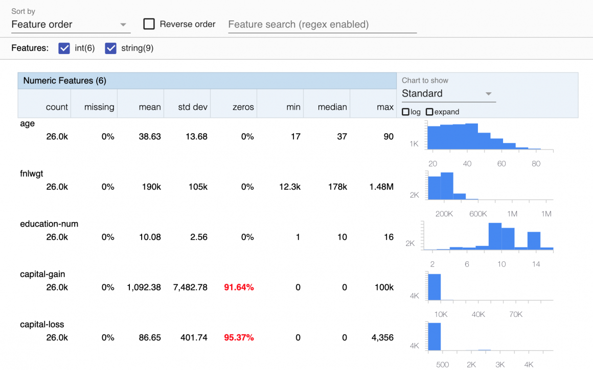
train_df_stats = tfdv.generate_statistics_from_dataframe(train_df)# tfdv.visualize_statistics(train_df_stats)

You should see the graphs describing each feature in detail:

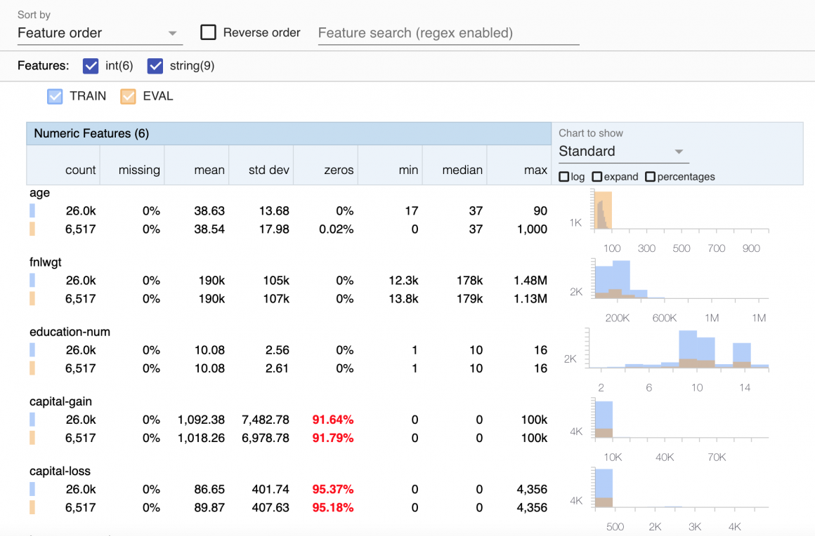
This graph is handy as it can show you how each feature is distributed and contains zeros, min, max, and other info. You can plot train and validation datasets together in the comparison mode, like so:

eval_df_stats = tfdv.generate_statistics_from_dataframe(eval_df) #calculate eval statistics 

tfdv.visualize_statistics(
    lhs_statistics=train_df_stats,
    rhs_statistics=eval_df_stats,
    lhs_name='TRAIN',
    rhs_name='EVAL'
)

And you should see charts like below:

Schema

When we’ve calculated statistics, we can infer the data specification that we (and TFX) will call Schema.

schema = tfdv.infer_schema(statistics=train_df_stats)
tfdv.display_schema(schema=schema)

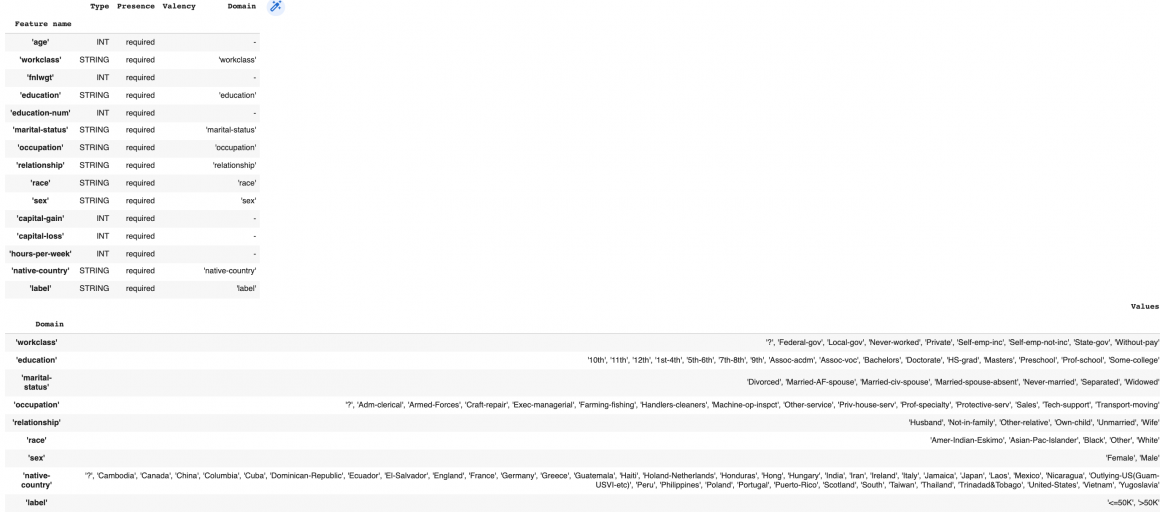
You should see the following data:

The Schema contains information about:

• data type: for example string, float, or integer;
• feature presence: if each datapoint is expected to have value for a specific feature;
• feature valency: how many values we can expect this feature to have;
• feature domains: expected values for a feature.

Schema is an important artifact that TFX would help us automatically build. You can also create your Schema definition and validate our data against it. The example of the code is below:

RAW_DATA_FEATURE_SPEC = dict(
    [ (name, tf.io.FixedLenFeature([], tf.string)) for name in CATEGORICAL_FEATURE_KEYS ] +
    [ (name, tf.io.FixedLenFeature([], tf.float32)) for name in NUMERIC_FEATURE_KEYS ] + 
    [ (name, tf.io.VarLenFeature(tf.float32)) for name in OPTIONAL_NUMERIC_FEATURE_KEYS ] + 
    [ (LABEL_KEY, tf.io.FixedLenFeature([], tf.string)) ]
)

SCHEMA = tft.tf_metadata.dataset_metadata.DatasetMetadata( 
      tft.tf_metadata.schema_utils.schema_from_feature_spec(RAW_DATA_FEATURE_SPEC) ).schema

We will define the expected Schema during subsequent phases of our automated Pipeline so that data validation happens automatically without human intervention.

You can work with the feature domain to add additional constraints or relax existing ones. For example, we could add additional common-sense restrictions to the ‘age’ feature. We can tell Schema that we expect it to be no less than 18 and no more than 100, like so:

tfdv.set_domain(schema, 'age', schema_pb2.IntDomain(name='age', min=18, max=100))

Data Validation

We have everything we need to validate our data now:

anomalies = tfdv.validate_statistics(statistics=eval_df_stats, schema=schema)
tfdv.display_anomalies(anomalies)

TFDV should find the following problems:

TFDV have spotted several inconsistencies:

• workclass: some datapoints are missing this value, and there are 2 values that are not in feature domain in Schema;
• age: two values are out of expected range;
• occupation: there are two unexpected values that are not in feature domain;
• native-country: there are four countries outside of expected domain;
• race: one value is not from the feature domain.

Now let’s soften requirements for ‘occupation’ and ‘workclass’ because we can tolerate minor deviations from the expected domain.

occupation_feature = tfdv.get_feature(schema, 'occupation')
occupation_feature.distribution_constraints.min_domain_mass = 0.9

workclass_feature = tfdv.get_feature(schema, 'workclass')
workclass_feature.distribution_constraints.min_domain_mass = 0.9

Next we can add new values to the ‘race’, ‘workclass’, ‘occupation’, and ‘native-country’ domains. This will contain a repeatable logic so that we can introduce a helper function:

def add_values_to_domain(values, domain, schema):
  domain = tfdv.get_domain(schema, domain)
  for value in values:
    domain.value.append(value)

This function will receive values to add, the name of the domain, and reference to the domain Schema. Withtfdv.get_domain, we will access the domain and append new values to it. Let’s use our helper function now:

new_race = ['Asian']
add_values_to_domain(new_race, 'race', schema)

new_workclass = ['Another new workclass', 'New workclass']
add_values_to_domain(new_workclass, 'workclass', schema)

new_occupation = ['Plumber', 'gamer']
add_values_to_domain(new_occupation, 'occupation', schema)

new_native_countries = ['Australia', 'Cameroon', 'Mongolia', 'Pakistan']
add_values_to_domain(new_native_countries, 'native-country', schema)

Let’s see if we managed to reduce the inconsistencies:

anomalies = tfdv.validate_statistics(statistics=eval_df_stats, schema=schema)
tfdv.display_anomalies(anomalies)

You should see only two problems remain:

And we only have missing values for ‘workclass’ and unexpected values for ‘age’ features. We understand that there is no way we would have guessed what would the correct values look like. So we will go ahead and remove these datapoints:

eval_df.dropna(inplace=True)

eval_df = eval_df[(eval_df.age <=90) & (eval_df.age >=17)]

And regenerate statistics:

eval_df_stats = tfdv.generate_statistics_from_dataframe(eval_df)

Let’s see if we have corrected all issues with the evaluation dataset.

anomalies = tfdv.validate_statistics(statistics=eval_df_stats, schema=schema)
tfdv.display_anomalies(anomalies)

You should see:

Conclusion

This article demonstrated how data ingestion and validation could look like in a semi-manual scenario. The algorithm downloaded and saved the data.

When data was downloaded, the program loaded it to the memory, calculated statistics of the data, and defined data Schema based on statistics.

With the Schema and statistics, we could check if there are problems with the new portion of data (evaluation dataset).

We fixed problems by either relaxing the restrictions or adding new values to the feature domain when we spotted issues.

In the following article, we will talk about Feature Engineering. First of all, we will review techniques that will help us define the optimal set of features. Then we will build an automated data transformation Pipeline for Production Machine Learning.

Next article in series – Optimizing Features in Production Machine Learning. Structured Dataset.