This article is part of a series describing Production ML – Production ML Series of Articles.
Neural Architecture Search and Model Tuning
Today we will talk about a fascinating topic: improving our model. And not just improve but create an automated algorithm that will:
- find an optimal architecture for our neural net,
- and the best set of hyperparameters automatically.
Neural Architecture Search is a reasonably new area, intending to develop a universal algorithm to find the best architecture for a model. This task is not simple to solve and computationally very expensive.
Hyperparameters optimization solves the problem of finding the best hyperparameters for a particular model. Best could mean different things in different situations. For example, it can be validation accuracy, precision, recall or f1 score, or anything else.
You can notice some commonalities between these two tasks, especially if we imagine a model architecture as a function from specific parameters. For example, it could be the number of dense layers in the model or the number of units in a particular dense hidden layer. We can decompose model architecture into parameters that will help you build the model architecture and work with them.
This is good news because now we can design a single solution (or an algorithm) for both problems. The researchers come up with many different solutions and will review only a subset of them. In particular, we will limit our review to three optimization methods:
- Random Search,
- Hyperband,
- Bayesian Optimization
Optimization Methods
Historically Grid Search was among the first methods that helped ML scientists find the best set of hyperparameters. The concept is straightforward: we have space of all possible variations of hyperparameters, and we cover it with a grid.
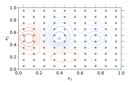
In the chart above, hyperparameters values are on x1 and x2. The circles drawn in the middle represent areas with the same optimization target value.
This way, we’re not testing all possible values for each parameter. Instead, we take every fifth or fifteenth potential value like on the picture above. This method reduces the computational burden (compared to trying all possible values). But it is also expensive.
To reduce the budget, researchers started using Random Search, which utilizes the same principle. We try only some options, not all. But instead of trying different parameters using a grid, we take them randomly (or almost randomly). So our search space looks like so:
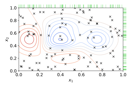
This method often works better than Grid Search but has some obvious downsides: reduced accuracy and the fact that it is still expensive.
The Hyperband method solves the problem with Random Search. It was introduced relatively recently (Hyperband: A Novel Bandit-Based Approach to Hyperparameter Optimization), but it already had proven to be one of the fastest optimization algorithms. We will see that it is faster than Random Search and Bayesian Optimization algorithms.
Under the hood, Hyperband uses Successive Halving and Asynchronous Successive Halving and sophisticated decision algorithm. In plain English, a very rough explanation could look like the following: we divide search space into two parts, take samples from both parts and compare results. The half with the best score will become our new search space, divide it in two, and so on. Again this is a very general explanation to understand the main principles.
Bayesian Optimization method calculates a probabilistic model that describes the mapping from values of hyperparameters to the optimization target value. In simple words, it tries to find the function that will tell the target’s most probable value for a particular set of hyperparameters.
Using this function, a tuner will test a limited amount of random values. Then it will focus on those parts of search space that are the most promising for getting us the best optimization target value. The search space will now look a bit differently:
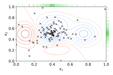
You will notice that the algorithm picks hyperparameters values not randomly. More samples are closer to the best model outcome. This way, the accuracy of the Bayesian Optimization algorithms tends to be a bit more accurate in some cases. However, it is not as fast as Hyperband.
An exciting area of research is a combination of Bayesian Optimization and Hyperband methods, but we will talk about it in further articles.
Keras Tuner
There are quite a few instruments for hyperparameter tuning and NAS. Most of them are based on Keras Tuner, a library with the most common hyperparameter tuning algorithms and tools.
All methods described above are included in the Keras Tuner library. We will use it extensively in this article. And first of all, let’s clarify some terms:
- Hyperparameters – any parameter of the model (including model architecture parameters);
- Tuner – the class that manages hyperparameters search process;
- Model Builder – a function that produces different variations of the model and its hyperparameters for the Tuner algorithm.
The model builder function will specify which parameters we want the Tuner to optimize. We will use an object that Keras Tuner will pass to the model builder function called ‘hp’. This object helps communicate the search space and how the Tuner should perform the search.
First of all, we initialize the hyperparameter, like so:
hyperp = hp.Int(‘test_hp’, min_value = 10, max_value = 100, step = 10)You can see that the hp object has methods (in this case method called ‘Int’). These methods are responsible for communicating the search space to the Tuner.
Some other methods we can use include:
- hp.Float() – sets the range of values with decimals (can be used to tune learning rate, for example);
- hp.Choice() – tuner will test specific values;
- hp.Boolean – choose between True or False.
The Tuner will work with the search space we will provide it through the hp object.
Sounds not too complex, right?
Then let’s write and run our code now.
Import Libraries
We will continue with the same dataset we used in the previous articles (Production ML: Model Training and Evaluation. Structured Dataset and Production ML Data Transformation Pipeline with Apache Beam. Structured Dataset.). There we transformed our dataset and prepared it for the training. We’ve also trained our model.
Now we will perform Neural Architecture Search to get the best f1 score. You can read more about the f1 score here – https://en.wikipedia.org/wiki/F-score. In simple words, the f1 score measures how often our model is right and how right our model is on average. Well, that probably might have confused you, so please read the article it will explain everything very detailed and clear way.
First of all, we will install TFX and Keras Tuner:
!pip install -U --quiet tfx
!pip install keras-tuner --quiet
If you follow along in colab, you need to restart your runtime.
We will import Tensorflow, TFX Transform, Keras Tuner, and utility libraries like os (working with files), math (making calculations), pprint (for friendly printing if we need it later).
import tensorflow as tf
print('TF: {}'.format(tf.__version__))

import tensorflow_transform as tft
print('Transform: {}'.format(tft.__version__))

import keras_tuner

import os
import math
import pprint
As in previous articles, we will specify the type of features we are working with.
CATEGORICAL_FEATURE_KEYS = [
    'workclass',
    'education',
    'marital-status',
    'occupation',
    'relationship',
    'race',
    'sex',
    'native-country',
]
NUMERIC_FEATURE_KEYS = [
    'age',
    'capital-gain',
    'capital-loss',
    'hours-per-week',
]
OPTIONAL_NUMERIC_FEATURE_KEYS = [
    'education-num',
]
ORDERED_CSV_COLUMNS = [
    'age', 'workclass', 'fnlwgt', 'education', 'education-num',
    'marital-status', 'occupation', 'relationship', 'race', 'sex',
    'capital-gain', 'capital-loss', 'hours-per-week', 'native-country', 'label'
]
LABEL_KEY = 'label'
And combine it to the dictionary that contains info about feature name, type, and value type.
RAW_DATA_FEATURE_SPEC = dict(
    [ (name, tf.io.FixedLenFeature([], tf.string)) for name in CATEGORICAL_FEATURE_KEYS ] +
    [ (name, tf.io.FixedLenFeature([], tf.float32)) for name in NUMERIC_FEATURE_KEYS ] +
    [ (name, tf.io.VarLenFeature(tf.float32)) for name in OPTIONAL_NUMERIC_FEATURE_KEYS ] +
    [ (LABEL_KEY, tf.io.FixedLenFeature([], tf.string)) ]
)
Set variables for the training loop:
#train model for 25 epochs
TRAIN_NUM_EPOCHS = 25
#set the number of train datapoints
#we will use it to calculate number of steps per epoch
NUM_TRAIN_INSTANCES = 32561
#set batch size (not too small for faster training)
TRAIN_BATCH_SIZE = 128
#set the number of train datapoints
#we will use it to calculate number of steps per epoch
NUM_TEST_INSTANCES = 16281

#we will ask algorithm to look for a files with a specific naming pattern
TRANSFORMED_TRAIN_DATA_FILEBASE = 'train_transformed'
TRANSFORMED_TEST_DATA_FILEBASE = 'test_transformed'

#and save model to a specific location
EXPORTED_MODEL_DIR = 'exported_model_dir'
Helper Functions
The first function we create will prepare data to feed the Tuner. It serves as a translator from TFT to TF Dataset, which we need for Tuner.
def _make_training_input_fn(tf_transform_output, transformed_examples, batch_size):

  def input_fn():
    return tf.data.experimental.make_batched_features_dataset(
        file_pattern=transformed_examples,
        batch_size=batch_size,
        features=tf_transform_output.transformed_feature_spec(),
        reader=tf.data.TFRecordDataset,
        label_key=LABEL_KEY,
        shuffle=True)

  return input_fn
The following function will calculate the f1 score. It receives the predicted labels and true labels and returns the f1 score value.
import keras.backend as K

def f1_metric(y_true, y_pred):
  #calculate true positives
  true_positives = K.sum(K.round(K.clip(y_true * y_pred, 0, 1)))
  #calculate all possible positives
  possible_positives = K.sum(K.round(K.clip(y_true, 0, 1)))
  #calculate predicted positives
  predicted_positives = K.sum(K.round(K.clip(y_pred, 0, 1)))
  #calculate precision
  precision = true_positives / (predicted_positives + K.epsilon())
  #calculate recall
  recall = true_positives / (possible_positives + K.epsilon())

  #get f1 score value
  f1_val = 2*(precision*recall)/(precision+recall+K.epsilon())

  return f1_val
The function below will save the best model for us.
def export_serving_model(tf_transform_output, model, output_dir):

  #add data transformation layer to the model
  model.tft_layer = tf_transform_output.transform_features_layer()

  #model is wraped with serving function
  #serving function is saved as a graph
  #tf.function works best with TensorFlow ops; NumPy and Python calls are converted to constants.
  @tf.function
  def serve_tf_examples_fn(serialized_tf_examples):
    #
    feature_spec = RAW_DATA_FEATURE_SPEC.copy()
    feature_spec.pop(LABEL_KEY)

    parsed_features = tf.io.parse_example(serialized_tf_examples, feature_spec)
    transformed_features = model.tft_layer(parsed_features)

    outputs = model(transformed_features)
    classes_names = tf.constant([['0', '1']])
    classes = tf.tile(classes_names, [tf.shape(outputs)[0], 1])

    return {'classes': classes, 'scores': outputs}

  concrete_serving_fn = serve_tf_examples_fn.get_concrete_function(tf.TensorSpec(
                                                                      shape=[None],
                                                                      dtype=tf.string,
                                                                      name='inputs'))

  signatures = {'serving_default': concrete_serving_fn}
  versioned_output_dir = os.path.join(output_dir, '1')

  #save the model
  model.save(versioned_output_dir, save_format='tf', signatures=signatures)
The function below orchestrates the entire process.
def train_and_evaluate(working_dir,
                       num_train_instances=NUM_TRAIN_INSTANCES,
                       num_test_instances=NUM_TEST_INSTANCES):

  #define train and test data path
  train_data_path_pattern = os.path.join( working_dir, TRANSFORMED_TRAIN_DATA_FILEBASE + '*')
  eval_data_path_pattern = os.path.join( working_dir, TRANSFORMED_TEST_DATA_FILEBASE + '*')

  #load transformed data
  tf_transform_output = tft.TFTransformOutput(working_dir)

  #initialize training dataset generator
  train_input_fn = _make_training_input_fn( tf_transform_output,
                                            train_data_path_pattern,
                                            batch_size = TRAIN_BATCH_SIZE)
  #load train data
  train_dataset = train_input_fn() ##

  #initialize evaluation dataset generator
  eval_input_fn = _make_training_input_fn( tf_transform_output,
                                           eval_data_path_pattern,
                                           batch_size = TRAIN_BATCH_SIZE)
  #load data for evaluation
  eval_dataset = eval_input_fn() ##

  #load feature spec
  feature_spec = tf_transform_output.transformed_feature_spec().copy()
  feature_spec.pop(LABEL_KEY) ##

  #prepare model input layers
  inputs = {}
  for key, val in feature_spec.items():
    if isinstance(val, tf.io.VarLenFeature):
      inputs[key] = tf.keras.layers.Input( shape=[None], name=key, dtype=val.dtype, sparse=True)
    elif isinstance(val, tf.io.FixedLenFeature):
      inputs[key] = tf.keras.layers.Input( shape=val.shape, name=key, dtype=val.dtype)
    else:
      raise ValueError('Feature data type is not supported: ', key, val)

  encoded_inputs = {} #
  for key in inputs:
    feature = tf.expand_dims(inputs[key], -1)
    if key in CATEGORICAL_FEATURE_KEYS:
      num_buckets = tf_transform_output.num_buckets_for_transformed_feature(key)
      encoding_layer = (tf.keras.layers.experimental.preprocessing.CategoryEncoding(
                                                                    num_tokens=num_buckets,
                                                                    output_mode='binary', sparse=False))
      encoded_inputs[key] = encoding_layer(feature)
    else:
      encoded_inputs[key] = feature

  #create model generator function
  def create_model(hp):
    #define hyperparameters
    num_hidden_layers = hp.Choice('num_hidden_layers', values=[4,6,10,14,18])
    num_units1 = hp.Choice('num_units1', values=[50,70,100,150])
    num_units2 = hp.Choice('num_units2', values=[30,50,70,100])
    num_units3 = hp.Choice('num_units3', values=[30,50])
    num_units4 = hp.Choice('num_units4', values=[20,30])
    num_units5 = hp.Choice('num_units5', values=[20,30])
    dropout_rate1 = hp.Choice('dropout_rate1', values=[0.5,0.8])
    dropout_rate2 = hp.Choice('dropout_rate2', values=[0.5,0.8])
    dropout_rate3 = hp.Choice('dropout_rate3', values=[0.1,0.5])
    dropout_rate4 = hp.Choice('dropout_rate4', values=[0.1,0.3])
    dropout_rate5 = hp.Choice('dropout_rate5', values=[0.1,0.3])

    #define model architecture
    #the loop will adjust the model architecture based on values of hyperparameters received from Tuner
    stacked_inputs = tf.concat(tf.nest.flatten(encoded_inputs), axis=1)

    for i in range(1, num_hidden_layers):
      if i == 1:
        output = tf.keras.layers.Dense(num_units1, activation='relu', kernel_initializer = 'he_uniform')(stacked_inputs)
        output = tf.keras.layers.BatchNormalization()(output)
        output = tf.keras.layers.Dropout(dropout_rate1)(output)
      if i == 2:
        output = tf.keras.layers.Dense(num_units2, activation='relu', kernel_initializer = 'he_uniform')(output)
        output = tf.keras.layers.BatchNormalization()(output)
        output = tf.keras.layers.Dropout(dropout_rate2)(output)
      if i == 3:
        output = tf.keras.layers.Dense(num_units3, activation='relu', kernel_initializer = 'he_uniform')(output)
        output = tf.keras.layers.BatchNormalization()(output)
        output = tf.keras.layers.Dropout(dropout_rate3)(output)
      if i == 4:
        output = tf.keras.layers.Dense(num_units4, activation='relu', kernel_initializer = 'he_uniform')(output)
        output = tf.keras.layers.BatchNormalization()(output)
        output = tf.keras.layers.Dropout(dropout_rate4)(output)
      if i >= 5:
        output = tf.keras.layers.Dense(num_units5, activation='relu', kernel_initializer = 'he_uniform')(output)
        output = tf.keras.layers.BatchNormalization()(output)
        output = tf.keras.layers.Dropout(dropout_rate5)(output)

    output = tf.keras.layers.Dense(2, activation='sigmoid')(output)
    model = tf.keras.Model(inputs=inputs, outputs=output)

    #compile model
    model.compile(optimizer='Adam',
                  loss='binary_crossentropy',
                  metrics=['accuracy', f1_metric])

    #give model to the Tuner
    return model


  #now we will initialize the Tuner
  #below you will see two options:
  # - Hyperband
  # - BayesianOptimization

  #faster option
  # tuner = keras_tuner.Hyperband(create_model,
  #                    objective=keras_tuner.Objective("f1_metric", direction="max"),
  #                    max_epochs=10,
  #                    factor=3,
  #                    directory='tuner',
  #                    project_name='tuner-demo',
  #                    overwrite=True)

  #slower
  tuner = keras_tuner.BayesianOptimization(create_model,
                     objective=keras_tuner.Objective("f1_metric", direction="max"),
                     max_trials=30,
                     directory='tuner',
                     project_name='tuner-demo',
                     overwrite=True)

  #tuning can be very expensive and time consuming
  #so we will instruct Tuner to stop if the objective metric is not changing
  #it will stop even if it didn't make all the trials we specified above
  stop_early = tf.keras.callbacks.EarlyStopping(monitor='f1_metric', patience=5)

  #perform hypertuning
  tuner.search(train_dataset,
               epochs=TRAIN_NUM_EPOCHS,
               steps_per_epoch=math.ceil(num_train_instances / TRAIN_BATCH_SIZE),
               callbacks=[stop_early])

  #get best hyperparameters
  best_hps = tuner.get_best_hyperparameters()[0]

  #print the results
  tuner.results_summary(1)
  # if you want to get specific params
  # print('num_hidden_layers: ', best_hps.get('num_hidden_layers'))
  # print('num_units1: ', best_hps.get('num_units1'))
  # print('num_units2: ', best_hps.get('num_units2'))
  # print('num_units3: ', best_hps.get('num_units3'))
  # print('num_units4: ', best_hps.get('num_units4'))
  # print('num_units5: ', best_hps.get('num_units5'))
  # print('dropout_rate1: ', best_hps.get('dropout_rate1'))
  # print('dropout_rate2: ', best_hps.get('dropout_rate2'))
  # print('dropout_rate3: ', best_hps.get('dropout_rate3'))
  # print('dropout_rate4: ', best_hps.get('dropout_rate4'))
  # print('dropout_rate5: ', best_hps.get('dropout_rate5'))

  #get best model
  best_model = tuner.get_best_models(num_models=1)[0]

  #save the best model
  exported_model_dir = os.path.join(working_dir, EXPORTED_MODEL_DIR) #
  export_serving_model(tf_transform_output, best_model, exported_model_dir)

  #evaluate model and return metric values
  metric_values = best_model.evaluate(eval_dataset, steps=num_test_instances)
  metric_labels = best_model.metrics_names

  return {label: val for label, val in zip(metric_labels, metric_values)}
Now let’s run the tuning process.
temp = '/content/drive/MyDrive/1Blog/tfx-series/transformed'

best_hps = train_and_evaluate(temp)
When tuning is done, you can see the best model was saved to the exported_model_dir.
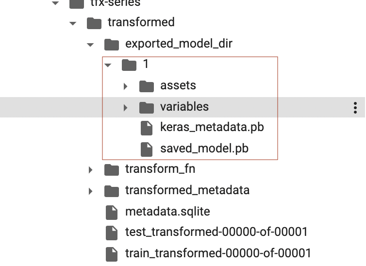
As well as information about trials tuner performed while searching the best model for us.
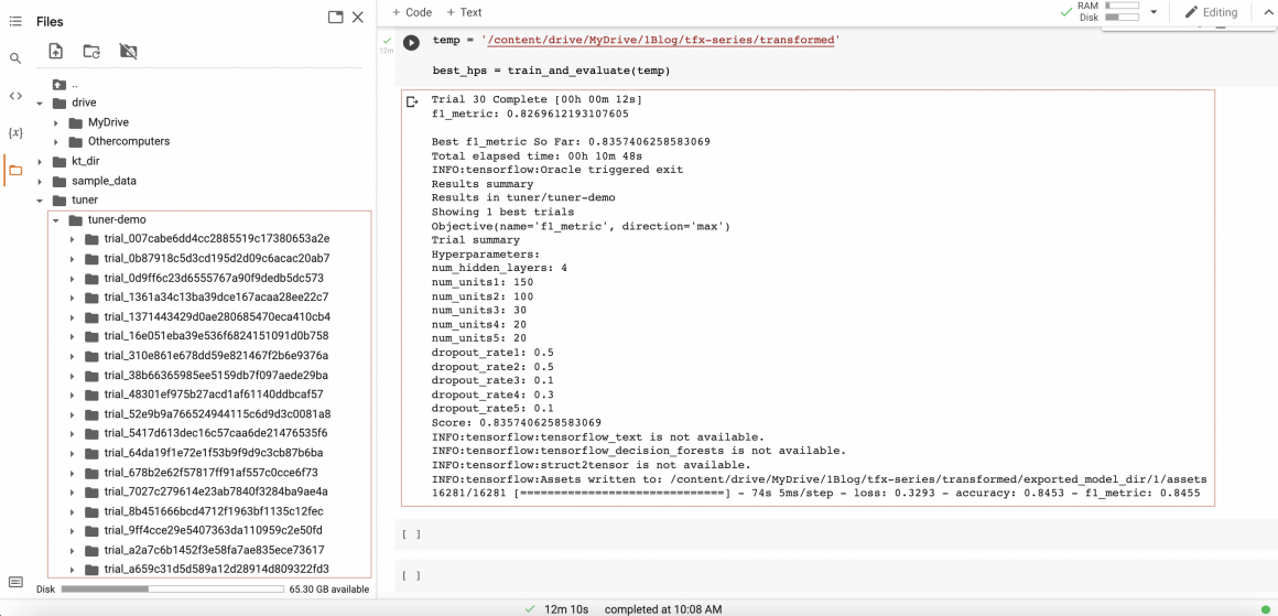
You can use this information for further analysis. For example, you can visualize it on Tensorfoard and analyze it.
%load_ext tensorboard
%tensorboard --logdir <path/to/log/directory>
When you run the code, you might get slightly different results. This is because of the stochastic way the algorithm will choose the starting point. We will get more stable and better results if we run more trials (here we run only 30). But it will take much more time.
In my experience, the production-grade tuning process can take from 4-5 hours to a few days.
Conclusion
NAS and hyperparameter tuning are exciting and vast topics. We’ve only scratched the surface, and I encourage you to dive deeper into this area.
In this article we:
- loaded pre-processed dataset,
- designed model builder function,
- initialized and launched Tuner.
I hope this article gave you a general idea of how you can use the Keras tuner to perform NAS and hyperparameter tuning for your projects.
I’ll do my best to explain this topic in more detail in further articles. So stay tuned, and may the Force be with you!


